TRFA Data Processor Advanced

Starting TRFA Data Processor Advanced
Time-resolved fluorescence and anisotropy data processor advanced (TRFA Data Processor Advanced) can be started via
v Start button on the Windows Task Bar:
? Go to the Programs/SSTC/TRFA Data Processor Advanced/ and click the 'TRFA Data Processor Advanced' item;
? Choose Run and specify the path to TRFADPAdv.EXE;
v Windows Explorer:
? Locate and double-click the TRFADPAdv.EXE file (if you have performed a default installation, this file is located in \Program Files\SSTC\TRFADP Advanced\Bin).

Take a look on a successfully loaded TRFA Data Processor Advanced

Main window
The view of the TRFA Data Processor Advanced Main Window without any experiments being opened is given on the following figure:

Main Window contains Main menu and Main toolbar.

Main menu
Main menu consists of the following popup items:
Items Description
File Contains menu commands for managing the experiments.
~~Tools~~ Contains menu commands for configuring active experiment and opening Databases.
Window Contains menu commands for managing the view of opened experiment windows and provides the ability to switch between them.
~~Help~~ Contains menu commands for accessing the online Help system and information about the copyright.

Main toolbar
The Main toolbar provides shortcuts for menu commands.

The correspondence between buttons and menu commands is the following:
Button Menu commands

File|New

File|Open

File|Save

Tools|Measurements DataBase

Tools|Experiments DataBase

Tools|Templates DataBase

Window|Cascade

Window|Tile

To find out more about the functionality of any Main toolbar button, click this button or the name of the corresponding Menu command in the table shown above.
The Main toolbar has short Help Hints. Help Hint is the pop-up text that appears when the mouse pointer passes over a toolbar button.

File menu
Use commands of the File menu for managing the experiments.
The File menu contains the following commands:
Commands Description

New Creates a new experiment.
Open Opens an Open an existing experiment dialog box for opening or finding an experiment.
Close Closes the active experiment without exiting the application.
Save Saves the active experiment. In the case if active experiment is saved for a first time, Save experiment as dialog box is opened.
Save As Opens Save experiment as dialog box for saving the active experiment with a different name.
Exit Finishes work with TRFA Data Processor Advanced.

Tools menu
The Tools menu contains the following commands:
Commands Description

Experimental configuration Opens the Configuration dialog box for configuring the currently active experiment.
Measurements Database Opens the Analysis Database Opens the Analysis Database.
Templates Database Opens the Templates Database.

Window menu
Use commands of this menu for managing the view of opened experiment windows and switching between them.
The Window menu contains the following commands:
Commands Description

Cascade Resizes and positions all windows in an overlapping pattern.
Tile Resizes and positions all windows in a non-overlapping pattern.
Arrange Icons Arranges icons of all minimized experiment windows.
Minimize All Minimizes all opened experiment windows.
Window List Displays the list of currently opened experiments. One can switch to required experiment by
(all items below clicking it's name.
the separator)

Help menu
Use commands of the Help menu to access the help system and get information about the copyright.
The Help menu contains the following commands:
Commands Description

Contents and Index Opens Help topic contents.
About Displays the copyright and version number for TRFA Data Processor Advanced.

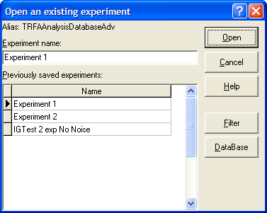
Open an existing experiment dialog box
Open an existing experiment dialog box is used to load a previously saved experiment.
An example view of the Open an existing experiment dialog box is given on the following figure:

To find out more about the functionality of any component, click this component on the figure.

Alias
Displays BDE Alias name associated with currently opened Analysis Database.

Experiment Name
Is used for entering the name of the experiment you want to load from the Analysis Database.
You can quickly find the experiment you want to load by typing the first few characters of its name. In this case the application will automatically select for you the first experiment that has the name with this few characters at the beginning.

Previously saved experiments
Displays the experiments previously saved in the Analysis Database.

Button "Help"
This button opens the help window that describes how to work with Open an existing experiment dialog box.

Button "Open"
This button finishes work with Open an existing experiment dialog box and loads the selected experiment.

Button "Cancel"
This button finishes work with Open an existing experiment dialog box without loading any experiments.

Button "Filter"
This button opens Filter.hlp>mainFilter dialog window, that allows to create the filter that can be applied to the Previously saved experiments list. If this filter is applied, the only experiment names that correspond to the filter criteria will be displayed.

Button "DataBase"
This button opens Analysis Database and sets the record selected in the Open an existing experiment dialog box as the current record in the Database.

Save experiment as dialog box
Save experiment as dialog box is used to save the active experiment with a different name.
An example view of the Save experiment as dialog box is given on the following figure:

To find out more about the functionality of any component, click this component on the figure.

Alias
Displays BDE Alias name associated with currently opened Analysis Database.

Experiment Name
Is used for entering the name for the experiment you are saving.

Previously saved experiments
Displays the previously saved experiments in the Analysis Database.

Button "Help"
This button opens the help window that describes how to work with Save experiment as dialog box.

Button "Save"
This button finishes work with Save experiment as dialog box and saves current experiment using selected name.

Button "Cancel"
This button finishes work with Save experiment as dialog box without saving the current experiment.

Button "Filter"
This button opens Filter.hlp>mainFilter dialog window, that allows to create the filter that can be applied to the Previously saved experiments list. If this filter is applied, the only experiment names that correspond to the filter criteria will be displayed.

Button "DataBase"
This button opens Analysis Database and sets the record selected in the Save experiment as dialog box as the current record in the Database.

Experiment window
Components of this window are used for creating and configuring an experiment, executing the analysis procedure and displaying the results.
Experiment window has two parts: Configuration part (left) and Analysis part (right).
An example view of the Experiment window is given on the following figure:

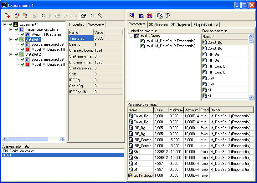
The Analysis part of the Experiment window consists of three pages:
? Parameters page is used for working with parameters.
? 3D Graphics page is used for displaying decays, weighted residuals and correlation functions of weighted residuals in three-dimensional space.
? 2D Graphics page is used for displaying decays, weighted residuals and correlation functions of weighted residuals in two-dimensional space.
? Fit quality criteria is used for displaying values and graphical dependencies of fit quality criteria calculated for data set currently selected in Configuration part .

Note
To choose the necessary page while working with TRFA Data Processor Advanced you should click on the corresponding Tab.

Configuration part of the Experiment window
This part of the Experiment window provides the quick access to the properties and parameters of the objects included in the current experiment and is responsible for displaying the information about the analysis progress.
An example view of the Experiment window Configuration part is given below:

To get more information about any area displayed on the picture above, simply click the left mouse button on it.

Configuration treeview
Configuration treeview displays the structure of the experiment and provides the access to any object included in it.
An example view of the Configuration treeview is given below:

The objects that can be displayed in this treewiev are divided into the following classes:

Experiment

Target fit criterion

Data Set

Data Source

Model

Instrumental response function

Reference compound

Background

Noise
The names of Experiment and Data Sets or additional information about Target fit criterion, Data Sources, Models, Instrumental response functions, Reference compounds, Backgrounds and Noises are displayed on the right of the corresponding object icon. A red dot

on the left of any object means that this object is modified. If the object is not modified the green tick

is displayed on the left of the given object. If the current object contains some child objects then it has one of the special indicators

. Press this indicator to show or hide the child objects.
Properties and parameters of the object, selected in the Configuration treeview, are displayed in the Properties and Parameters tables, correspondingly.

Parameters table
This table is used to display the names and the values of the parameters related the object currently selected in the Configuration treewiev.
An example view of the Parameters table is given below:

Note
To choose the Properties table you should click on the properties tab.

Properties table
Local menu

This table is used to display the names and the values of the properties related the object currently selected in the Configuration treewiev.
An example view of the Properties table is given below:

Note
To choose the Parameters table you should click on the parameters tab.

Analysis information window

This window monitors the information about the analysis progress.
An example view of the Analysis Information window is given below:

The new information in this window appears in the following cases:
? after value of Target fit criterion (for example Chi-square) was calculated;
? while the fit is running;
? while the analysis of the confidential intervals is running.

Templates
Template contains the all information (the types of the models and their properties, settings and links of the parameters being estimated) that is related to the analysis of the Data Sets within the current experiment. Template provides the quick way for analyzing the large amount of data with the same analysis scheme.

Properties
Properties are the values that are used for configuring the corresponding object within the current experiment.

Parameters
Parameters are the values that can be estimated during the analysis. Each parameter can be fixed into the predefined value. For each parameter the range of admissible values can be set by defining the constraints.

Parameter constraints
The parameter constraints serve to limit the change of the parameter value in admissible range during the fit.

The simple way to limit the range where the value of the fit parameter can be varied is to set minimum and maximum values for this parameter. This can be done via Parameters setting table.

In order to create more complex parameter constraints TRFA Data Processor Advanced supports the ability to construct functional relationships between parameters that belong to the same model. Such constraints are represented in the software as separate objects that can be added to the models. The constraint object can operate with any parameters according to its formula and therefore is independent on type of the model.

Now the following functional constraints are available to be used with TRFA Data Processor Advanced:
1. Ratio.

To manage functional constraints within the model use Add/Remove constraints dialog box available via Constraints property of the model.

External parameters
External parameters are the values that describe the conditions of the fluorescence decay measurement. These parameters cannot be fitted but are required by some models to calculate theoretical decays.

Total fluorescence decay
The term 'total fluorescence decay' is used to denote the fluorescence decay measured on magic angle (vertically polarized excitation and emission polarizer oriented 54.7 degrees from vertical).

Parallel fluorescence decay
The term 'parallel fluorescence decay' is used to denote the fluorescence decay measured when both excitation and emission polarizers are oriented vertically.

Perpendicular fluorescence decay
The term 'perpendicular fluorescence decay' is used to denote the fluorescence decay measured when excitation polarizer is oriented vertically and emission polarizer is oriented horizontally.

Fit quality criteria
The fit quality criteria together with the value of Target fit criterion are intended for judging the quality of the fit. All these criteria can be divided into two large groups:
1. Numerical fit quality criteria. After being calculated these fit quality criteria return the numerical values that can help to make decision about the quality of the fit. The following numerical fit quality criteria are implemented in TRFA Data Processor Advanced:

Standard normal deviation (Zc2);

Durbin Watson parameter;

Runs Test.
2. Graphic fit quality criteria. After being calculated these fit quality criteria return the graphical dependencies that can be used for judging the quality of the fit. The following graphic fit quality criteria are implemented in TRFA Data Processor Advanced:

Weighted residuals;

Autocorrelation function of the residuals;

Heterosedasticity of the residuals;

Normal probability density function of the residuals.

The values of fit quality criteria are generated each time after fit is done or Target fit criterion is calculated.

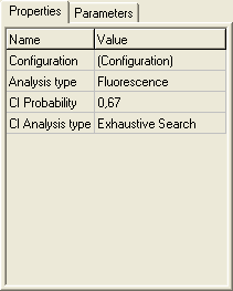
Experiment
In the TRFA Data Processor Advanced the notion Experiment means the numerical experiment. Within the TRFA Data Processor Advanced the Experiment is associated with a special object.
Experiment Object contains all other objects that are used for preparation of data and analysis execution.
Experiment icon is following:

.

Experiment properties:
1. Configuration provides access to Configuration dialog box. Press the button on the right side of the property value box to open this dialog box.
2. Analysis type allows to choose the type of analysis to be executed.
Fluorescence analysis type should be used either for analysis of fluorescence decays measured at magic angle or in the case when total fluorescence calculated from parallel and perpendicular polarization components is analyzed.
Anisotropy analysis type is applied for recovering anisotropy parameters in the case if Data Set contains both parallel and perpendicular polarization components.
3. CI Probability specifies the value of confidential probability.
Minimum possible value is 0.001.
Maximum possible value is 0.999.
Default value is 0,67.
4. CI Analysis type allows to select a method for confidential intervals analysis. The following CI Analysis types are currently available: Exhaustive search and Standard errors.

Target fit criterion
Target fit criterion Object is used to calculate the numerical value that shows degree of conformity of measured (simulated) and theoretical decays. This value is used by optimization method to find the estimations of fit parameters.
Target fit criterion icon is following:

.

Now the following target fit criteria are available in TRFA Data Processor Advanced:
1. Chi-square;
2. Maximum-Likelihood with Poissonian statistics.

Optimization method
Optimization method Object is used to find the values of fit parameters that correspond to the minimum value of target fit criterion and thus ensure the best conformity of measured (simulated) decays and theoretical decays generated by models.

The fitting procedure included in TRFA Data Processor Advanced is based on the Marquardt-Levenberg optimization method [13, 16].

Data Set
Data Set Object contains all necessary information that describes the data, related to the one measurement (simulation). It contains data for sample decay, Instrumental response function or Reference decay and Background (in the case it is available). In the case if data come from polarization experiment Data Set may contain either both parallel and perpendicular components or separately one of them. Also Data Set contains values that define the conditions under which the data will be analyzed.
Data Set icon is following:

.

Data Set properties:
1. Time Step indicates the width of the channel for measured (simulated) fluorescence decay. The value of this property is calculated as original time channel width that was set during measurement (simulation) multiplied on the value of Binning property. This property is read only if Data Set contains measured data, otherwise it is changeable.
2. Binning allows to join the values of measured (simulated) data taken from two or more neighboring channels. The value of this property must be integer and indicates the number of united channels.
3. Channels count indicates the total number of points in the measured (simulated) data. The value of this property is calculated as original number of points that was set during measurement (simulation) divided on the value of Binning property. This property is read only if Data Set contains measured data, otherwise it is changeable.
4. Start analysis at defines the initial point for analysis. The characteristic contained in the Data Set will be analyzed starting at this point.
Minimum possible value is 0.
Maximum possible value equals to End analysis at.
5. End analysis at defines the end point for analysis.
Minimum possible value equals to the Start analysis at.
Maximum possible value is Channels count - 1.
Default value is Channels count - 1.
6. Start criterion at specifies the initial point for the Target fit criterion calculation.
Minimum possible value equals to the Start analysis at.
Maximum possible value is Channels count - 1.
Default value equals to the Start analysis at.
7. Ref. life time shows the value that is used as initial guess for tau_ref parameter that corresponds to the life time of single exponential reference compound. By default the value of this property is loaded from Measurements Database. This property is available only for data sets that contain reference compound data.
8. G-Factor shows the value of G-Factor that is used for combining sample and reference compound parallel and perpendicular polarization components to the total decay. By default the value of this property is loaded from Measurements Database. This property is available only for data sets that contain parallel and perpendicular polarization components.
9. Scatter G-Factor shows the value of G-Factor that is used for combining Instrumental response function parallel and perpendicular polarization components to the Instrumental response function. By default the value of this property is loaded from Measurements Database. This property is available only for data sets that contain parallel and perpendicular polarization components and Instrumental response function data.
10. Shift (Parallel Shift and Perpendicular Shift) shows the value of shift between sample decay and Instrumental response function expressed in time channels. By default the values of these properties are loaded from Measurements Database. In the case if data set contains parallel and perpendicular polarization components two properties Parallel Shift and Perpendicular Shift are available. Otherwise one property Shift is present. The value of Shift property is used as initial guess for shift parameter.
11. IRF/REF Bg (Par. IRF/REF Bg and Perp. IRF/REF Bg) shows the level of time-independent background in Instrumental response function or Reference compound. By default the values of these properties are loaded from Measurements Database. In the case if data set contains parallel and perpendicular polarization components two properties Par. IRF/REF Bg and Perp. IRF/REF Bg are available. Otherwise one property IRF/REF Bg is present. The value of IRF/REF Bg property is used as initial guess for IRF/REF_Bg parameter.
12. TC Bg factor (Par. TC Bg factor and Perp. TC Bg factor) show the values that are used as initial guesses for TCBg_factor (TCBg_factor_par and TCBg_factor_perp) parameters that correspond to the multiplication factors for time dependent background (time dependent background parallel and perpendicular polarization components). These parameters allow taking into account difference in measurement time between sample and background. For example, if sample decay was measured two times longer than background then TC Bg factor is 2. By default the values of these properties are loaded from Measurements Database. These properties are present only for data sets that contain measured or simulated background data. In the case if data set contains parallel and perpendicular polarization components two properties Par. TC Bg factor and Perp. TC Bg factor are available. Otherwise one property TC Bg factor is present.
13. Const Bg (Par. const Bg and Perp. const Bg) show the values that are used as initial guesses for Const_Bg (Const_Bg_par and Const_Bg_perp) parameters that correspond to the level of time-independent background in sample total decay (sample parallel and perpendicular polarization components). By default the values of these properties are loaded from Measurements Database. In the case if data set contains parallel and perpendicular polarization components two properties Par. const Bg and Perp. const Bg are available. Otherwise one property Const Bg is present.
14. IRF Contrib. (Par. IRF Contrib. and Perp. IRF Contrib.) show the values that are used as initial guesses for IRF_Contrib (IRF_Contrib_par and IRF_Contrib_perp) parameters that take into account scattered light contribution in sample total decay (sample parallel and perpendicular polarization components). By default the values of these properties are loaded from Measurements Database. These properties are present only for data sets that contain measured or simulated Instrumental response function data. In the case if data set contains parallel and perpendicular polarization components two properties Par. IRF Contrib. and Perp. IRF Contrib. are available. Otherwise one property IRF Contrib. is present.

Data Source
Data Source Object is used to prepare the source data for the analysis.
Data Source can be Measured or Simulation.
Measured Data Source is used for preparation of measured data.
Simulation Data Source is used to generate data on the bases of Model, Instrumental response function or Reference, Background and Noise.
Data Source icon is following:

.

Data Source properties:
This object does not have any properties.

Model
To analyse fluorescence decays with TRFA Data Processor Advanced one should select appropriate mathematical model that will describe experimental data. All models in TRFA Data Processor Advanced are based on the general equations. The form of these equations depends on the both type of the data located in the data set and the type of the analysis.

All models can be applied for both analysis of single fluorescence decays and global analysis of more than one fluorescence decay. Also some models can be used to perform anisotropy analysis.

In TRFA Data Processor Advanced the models are represented by the corresponding Model Objects. Model Object can belong either to the Data Set or to the Simulation Data Source. In the first case Model is used to generate the theoretical fluorescence decay. In the second case it is used to generate noise-free source fluorescence decay.
Model icon is following:

.

The models can have properties that are used to change the model configuration.
Properties common for all models:
1. Constraints provides access to ~~Add/Remove constraints dialog box~~. Press the button on the right side of the property value box to open this dialog box.

The shape of theoretical fluorescence decay generated by the model depends on the values of fit parameters that can be estimated during the fit. Some of these parameters are the same for all models and originate from the general model equations defined by the choosen analysis type.The list of common model parameters depends on the type of the data located in the data set that is associated with the model.
Fit parameters common for all models:
- for data set with non-polarized data:
1. Shift is the shift between Instrumental response function and sample fluorescence decay expressed in time channels (see D in the analysis of single fluorescence decays section). This parameter is available only for data sets that contain Instrumental response function;
2. IRF/REF_Bg is a time-uncorrelated background in the Instrumental response function or Reference compound decay (see b in the analysis of single fluorescence decays section);
3. TCBg_factor is relative weight coefficient of background emission (see g in the analysis of single fluorescence decays section). This parameter is available only for data sets that contain Bacground;
4. Const_Bg is a time-uncorrelated background in the sample decay (see c in the analysis of single fluorescence decays section);
5. IRF_Contrib is a coefficient of scattered light contribution (see n in the analysis of single fluorescence decays section). This parameter is available only for data sets that contain Instrumental response function;
6. tau_ref is a decay time of one-exponential Reference compound decay (see

in the analysis of single fluorescence decays section). This parameter is available only for data sets that contain Reference compound decay.
- for data set with polarized data:
1.TCBg_factor_par and TCBg_factor_perp are relative weight coefficients of background emission for parallel and perpendicular polarization decay components respectively (see

and

in the anisotropy analysis section) . These parameters are available only for data sets that contain Bacground;
2. Const_Bg_par and Const_Bg_perp are time-uncorrelated background levels in the sample parallel and perpendicular polarization decay components respectively (see

and

in the anisotropy analysis section);
3. IRF_Contrib_par and IRF_Contrib_perp are coefficients of scattered light contribution for parallel and perpendicular polarization decay components respectively (see

and

in the anisotropy analysis section). These parameters are available only for data sets that contain Instrumental response function;
4. tau_ref is a decay time of one-exponential Reference compound decay (see

in the anisotropy analysis section). This parameter is available only for data sets that contain Reference compound decay.

Now the following models are available to be used with TRFA Data Processor Advanced:
1. Multi-exponential;
2. Anisotropy;
3. Poisson distribution of decay rates;
4. Gauss distribution of decay rates;
5. 2-compartmental;
6. 3-compartmental.

Instrumental response function
Instrumental response function Object is used for data simulation and represents response of the experimental equipment at excitation wave length in the case when measured sample is replaced by appropriate scatterer.
Instrumental response function icon is following:

.

Now the following instrumental response functions are available to be used with TRFA Data Processor Advanced:
1. Measured. In this case simulation procedure uses measured data as instrumental response function for generating simulated fluorescence decay. The data of instrumental response function can be loaded from Measurements Database.
2. Simulated. In this case instrumental response function is generated by the following equation:

Instrumental response function properties:
1. Pulses count defines number of excitation pulses that will be simulated during the simulation time period. The time between neighboring excitation pulses is calculated by division of the simulation time period on number of excitation pulses. This property is available only for simulated instrumental response function in the case if simulation data is configured to generate multiexcitation decays.
2. PercentStandoff defines the length in percent of zero level section of instrumental response function located at the beginning of time scale.
3. A defines the value of parameter A in the equation for simulated instrumental response function mentioned above. This property is available only for simulated instrumental response function.
4. B defines the value of parameter B in the equation for simulated instrumental response function mentioned above. This property is available only for simulated instrumental response function.

Reference compound
Reference compound Object is used for data simulation and represents the fluorescence decay of reference compound that can be used instead of Instrumental response function for calculating theoretical curve similar to one obtained from real measurements.
Reference compound icon is following:

.

Now the following reference compounds are available to be used with TRFA Data Processor Advanced:
1. Measured. In this case simulation procedure uses measured data as reference compound for generating simulated fluorescence decay. The data of reference compound can be loaded from Measurements Database.
2. Simulated. In this case reference compound is generated by the following equation:

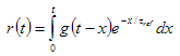
where

is reference lifetime.

Reference compound properties:
This object does not have any properties.

Background
Background Object is used for data simulation and represents background noise.
Background icon is following:

.

Now the following background types are available to be used with TRFA Data Processor Advanced:
1. Measured. In this case simulation procedure uses measured data as background for generating simulated fluorescence decay. The data of background can be loaded from Measurements Database.
2. Simulated. In this case time independent background is generated at average level specified by user.

Background properties:
1. Level defines the average amplitude level of time independent background. This property is available only for simulated background.

Noise
Noise Object is used for data simulation and adds poissonian noise to the fluorescence decay curve generated by Model, instrumental response function, Reference compound and Background. Before adding statistical noise to the fluorescence decay curve generated by Model, instrumental response function and Reference compound these curves are rescaled to the maximum values defines by corresponding property of Noise Object (see list bellow). The amplitude level of Background is defined by its own property. The noise addition procedure consists in replacing the undistorted value of certain curve at given time point with the realization of poissonian random value with mean equal to the undistorted value.
Noise icon is following:

.

Noise properties:
1. Sample max specifies the level to which the maximum of the simulated sample decay is rescaled before adding the statistical noise.
2. IRF max specifies the level to which the maximum of the instrumental response function is rescaled before adding the statistical noise. This property is available in the case if instrumental response function is present in simulated data set.
3. REF max specifies the level to which the maximum of the Reference compound is rescaled before adding the statistical noise. This property is available in the case if Reference compound is present in simulated data set.

Parameters page
This page is used to manage the settings of the fit parameters and parameters linkage.
An example view of the Parameters page is given below:

The following components are related to the Parameters page:
Parameters toolbar
Linked parameters treeview
Free parameters list
Parameters settings table
Click the corresponding item to get more information about it.

Linked parameters treeview
Local menu

Linked parameters treeview is used for linking parameters and displaying the linked parameter groups. To find out more about how to link and unlink parameters see Linking parameters and Unlinking parameters operations.
An example view of the Linked parameters treeview is given below:

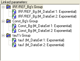
Parameter groups are marked with the following icon:

.
Parameters are marked with the following icons:

and

.
The names of the parameter groups and parameters are displayed on the right of the corresponding icons.
If the current parameter group contains some parameters then it has one of the special indicators

. Press this indicator to show or hide the parameters related to the current parameter group.

Free parameters list
Local menu

Free parameters list displays all free (unlinked) parameters within the experiment.
An example view of the Free parameters list is given below:

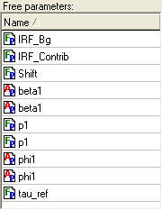
The parameters that are displayed in this list are sorted by name. To change the sorting direction of the parameters contained in the Free parameters list click on the list header. A small triangle located on the right of the header name shows the sort direction.

The free parameters that are going to be linked will be moved from this list to the Linked parameters treeview. The linked parameters that are going to be unlinked will be moved from the Linked parameters treeview to Free parameters list.
To find out more about how to link and unlink parameters see Linking parameters and Unlinking parameters operations.

Parameters settings table
Local menu

This table displays the settings of the parameters and parameter groups related to the current experiment.
An example view of the Parameters settings table is given bellow:

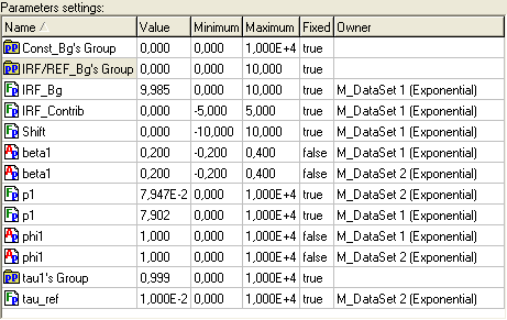
Parameters settings table contains the following fields:
Field Name Description

Name Contains the name of the parameter or parameter group. It can be changed only for parameter groups.
Value Contains the value of the parameter or parameter group. It can vary from the minimum value contained in the field Minimum to the maximum value contained in the field Maximum.
Minimum Contains the minimum possible value of the parameter or parameter group.
Maximum Contains the maximum possible value of the parameter or parameter group.
Fixed Indicates whether the value of the current parameter or parameter group should be optimized during the analysis. If Fixed is true then the value of the current parameter will be constant during the analysis, otherwise the parameter will participate in the fit.
CI Left,
CI Right Contain left and right bounds of Confidential Interval, which was obtained for the current parameter or parameter group if Confidential Interval analysis was performed for it. These fields are read only.
CI Analysis Indicates whether the Confidential Interval should be calculated for the current parameter or parameter group. If button CI Analysis on the Configuration toolbar is down and CI Analysis value is true then the Confidential Interval will be calculated for the current parameter or parameter group while Confidential Interval Analysis is executed.
Owner Contains the Name of the model, which generated the current parameter (for parameters only). It is read only.

Notes
? Fields CI Left, CI Right, CI Analysis are visible only if button CI Analysis is down on the Configuration toolbar.
? The parameters that are displayed in this table can be sorted by any field. To perform the sorting by the given field, click the header of the appropriate column. To change the sorting direction of the parameters click a second time on the same header. A small triangle located on the right of the header name shows the sort direction.

Parameter group
In TRFA Data Processor Advanced the special object parameter group is used for linking parameters. The parameters that belong to one parameter group are considered as linked to each other. Parameter groups are displayed in the Linked parameters treeview.

Unlinking parameters

To unlink any parameter and make it free select the parameter you want to unlink in Linked parameters treeview, drag it and drop on the Free parameters list.

To unlink all parameters related to the given parameter group:
? Select the current group in the Linked parameters treeview or Parameters settings table.
? Press right mouse button on the selection to display the local menu and select the Empty local menu command.

If you want to delete the given parameter group while freeing all it's parameters, then you should use the Delete local menu command instead of Empty local menu command. The same operation for the parameter group currently selected in the Linked parameters treeview can be done using Delete selected parameter group button of the Parameters toolbar.

Linking parameters
In TRFA Data Processor Advanced the special object parameter group is used for linking parameters. The parameters that belong to one parameter group are considered as linked to each other.
To link two or more parameters together you should perform the following steps:
1. Create the new parameter group. There are some ways to create parameter group:
? Press the button Create new parameter group on the Toolbar of the Parameters page;
? Right click on the Linked parameters treeview to open it's local menu. Choose New group menu command from this local menu.
2. Select the parameters you want to link in Free parameters list, drag them and drop on the newly created group.

If you have previously created parameter groups you can add any free parameter(s) to any of these groups.
Also, you can use local menu commands Link To, Link all [parameter name]'s of Free parameters list or Parameters settings table as an alternative way for linking parameters.

2D Graphics page
This page is used to display fluorescence and anisotropy decays, Instrumentsl response function, background, weighted residuals and their autocorrelation function in two-dimensional space.
The following components are related to the 2D Graphics page:
Toolbar
2D Fluorescence, Residuals and Autocorrelation boxes
An example view of the 2D Graphics page is given below:

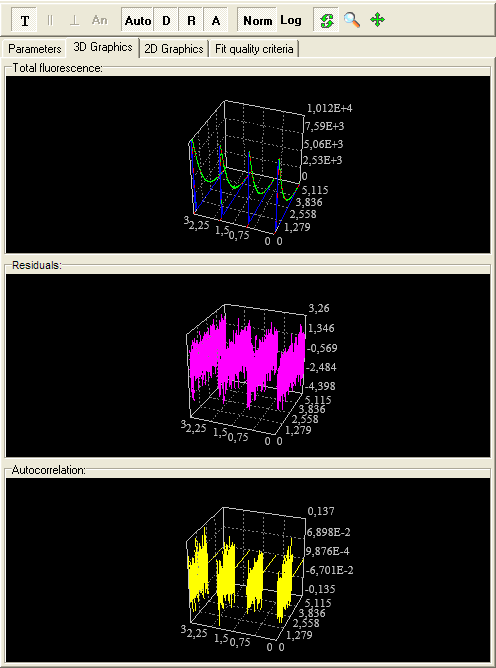
3D Graphics page
This page is used to display fluorescence and anisotropy decays, Instrumentsl response function, background, weighted residuals and their autocorrelation function in three-dimensional space.
The following components are related to the 3D Graphics page:
Toolbar
3D Fluorescence, Residuals and Autocorrelation boxes
An example view of the 3D Graphics page is given below:

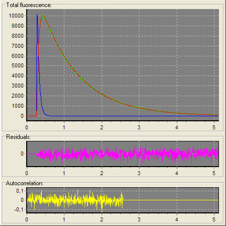
2D charts
Local menu

2D Fluorescence chart displays measured (green) and theoretical (red) fluorescence (anisotropy) decays, Instrumental response function (reference compound), Background in two-dimensional space. 2D Residuals chart displays weighted residuals in two-dimensional space. 2D Residuals autocorrelation chart displays weighted residuals autocorrelation function in two-dimensional space.
2D charts display curves according to the selection in the Configuration treeview. If the Experiment object is selected in the Configuration treeview then the curves related to all Data Sets within the current Experiment are displayed in 2D charts. If any Data Set or child objects (Data Source, Model, Noise, etc.) are selected then the only curves that belong to this Data Set are displayed in 2D charts.

An example view of the 2D charts is given below:

For 2D chart you can:
? move curves in the box by keeping the right mouse button down and moving the mouse pointer through the chart.
? zoom in the image by dragging the cursor diagonally across the necessary area from left top corner to right bottom corner.
? restore whole view of the image by pressing left mouse button and dragging mouse pointer on some positions to upper left.
Additional actions with 2D Chart available through the local menu.

3D charts
Local menu

3D Fluorescence chart displays measured (green) and theoretical (red) fluorescence (anisotropy) decays, Instrumental response function (reference compound), Background in three-dimensional space. 3D Residuals chart displays weighted residuals in three-dimensional space. 3D Residuals autocorrelation chart displays weighted residuals autocorrelation function in three-dimensional space.

3D charts display all curves within the current experiment. Here the curves sequence corresponds to the Data Sets sequence in the Configuration treeview.
An example view of the 3D charts is given below:

For 3D chart you can rotate, zoom or move the 3D image by keeping the left mouse button down and moving the mouse pointer through the 3D chart. The active transformation of 3D image depends on the mode that is set through the Toolbar or the Chart3DConfigDlg.hlp>main3D chart configuration dialog box.

Additional actions with 3D Chart available through the local menu.

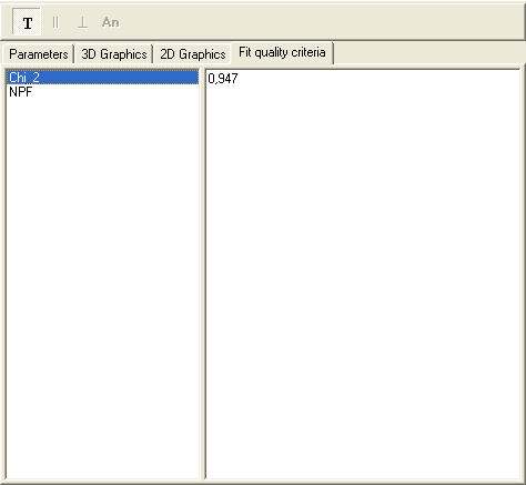
Fit quality criteria page
This page is used to display the values for text fit quality criteria and graphs for graphical fit quality criteria that are used to estimate the quality of the fit within current experiment. If any Data Set or child objects (Data Source, Model, Noise, etc.) are selected
The Fit quality criteria page displays information according to the selection in the Configuration treeview. If any data set or one of its child objects (Data Source, Model, Noise, etc.) are selected then fit quality criteria values (graphical dependencies) are displayed for this data set. Otherwise the Fit quality criteria page is not available.

An example views of the Fit quality criteria page is given below:

To find out more about the functionality of any component, click this component on the figure.

Fit quality criteria list
Displays the list of fit quality criteria that were added to the current experiment and were calculated after the fit.

Text fit quality criteria values
Displays the values that correspond to the text fit quality criterion currently selected in the fit quality criteria list.

Graphic fit quality criterion chart
Displays the curves that correspond to the graphic fit quality criterion currently selected in the fit quality criteria list.

Local menus
TRFA Data Processor Advanced offers local menus (context menus) for several interface elements. All these menus can be opened through a right mouse click when mouse pointer is over the element that contains local menu.

Local menu of the Configuration treeview

This local menu contains following items:
1. Rename
2. Export Data
3. Apply Template
4. Save Template
5. Simulate
6. Execute
7. Stop
8. Calculate Chi-square
9. Show Properties
10. CI Analysis
11. Configuration

Local menu command: Export Data
This menu command opens Export data dialog box that allows exporting the data from any Data Set within the current experiment to the text file.

Local menu command: Simulate
This menu command executes the simulation procedure to prepare the source data in the Simulation Data Sets.

Local menu command: Apply Template
This menu command opens the Load and apply an existing template dialog box for applying the previously saved template to the current experiment.

Local menu command: Execute
This menu command executes the fit.

Local menu command: Save Template
This menu command opens the Create and save new template dialog box for creating a new template and saving it to the Templates Database.

Local menu command: Stop
This menu command interrupts the fit.

Local menu command: Calculate Chi-square
This menu command calculates Chi-square for the current values of fit parameters. Also theoretical curves and residuals curves will be built and displayed in the corresponding graphical windows.

Local menu command: Show properties
If this menu item is checked properties and parameters tables are shown, otherwise they are hidden.

Local menu command: Configuration
This menu command opens the Experiment configuration window for configuring the current experiment.

Local menu command: CI Analysis
If this menu item is checked confidential intervals for the estimated parameters will be calculated after execution of the fit.

Local menu command: Rename
This menu command allows to change the name of the Experiment or Simulation Data Sets. The Rename menu command appears only if the Experiment or Simulation Data Set object is selected in the Experiment configuration treeview. After you have chosen this menu command the inplace editor will be displayed instead of the selected treeview node.

Local menu of the Properties table

This local menu contains following items:
1. Apply to all similar objects

Local menu command: Apply to all similar objects
This menu command allows to set the value of the currently selected property to the same properties of all similar objects within the current experiment.

Local menu of the Linked parameters treeview

This local menu contains following items:
   1. Rename
   2. Empty
   3. Delete
   4. Expanded
   5. Link To
   6. Position
   7. New Group

Local menu command: Rename
This menu command allows to rename parameter group selected in Linked parameters treeview. After you have chosen this menu command the inplace editor will be displayed instead of the selected treeview node.

Local menu command: Empty
This menu command empties the parameter group currently selected in the Linked parameters treeview and moves all its parameters to the Free parameters list. Execution of this command is equivalent to the unlinking the parameters contained in this group.

Local menu command: Delete
This menu command deletes the parameter group currently selected in the Linked parameters treeview and moves all its parameters in the Free parameters list. Execution of this command is equivalent to the unlinking the parameters contained in this group and deleting the current parameter group.

Local menu command: Expanded
If this menu item is checked the parameters related to the current parameter group are visible.

Local submenu: Link To
This submenu contains local menu commands that provide the ability to relink the selected parameter or parameter group to any other parameter group. The name of the submenu command is equivalent to the name of the target parameter group.

Submenu command: Position
This submenu contains local menu commands that are used for changing the position of the selected parameter within the given parameter group or the position of any parameter group within the current experiment. This submenu contains the following commands:
Move Up - moves the selected parameter or parameter group one position up.
Move Down - moves the selected parameter or parameter group one position down.
Place First - places the selected parameter or parameter group to the first position in the list.
Place Last - places the selected parameter or parameter group to the last position in the list.

Local menu command: New Group
This menu command creates new parameter group within the current experiment.

Local menu of the Free parameters list

This local menu contains following items:
1. Link all [parameter name]'s
2. Link To
3. Find Model
4. View on graph

Local menu command: Link All
This menu command creates new parameter group with name "[parameter name]'s Group" and moves all parameters with the name [parameter name] to this newly created parameter group.

Note
[parameter name] - is the name of the first parameter in the selection.

Local submenu: Link To
This submenu contains local menu commands that provide the ability to link the selected parameter(s) to any existing parameter group. The name of the submenu command is equivalent to the name of the target parameter group.

Local menu command: Find Model
This menu command finds and selects model in the Configuration treeview which contains the parameter currently selected in the Free parameters list. This local menu command is visible if only one parameter is selected in the Free parameters list.

Local menu command: View on graph
This menu command opens "Fit parameter vs. data set number view" window.

Local menu of Parameters settings table

This local menu contains following items:
   1. Rename
   2. Empty
   3. Delete
   4. Link all parameter name's
   5. Link To
   6. Find Model
   7. View on graph
   8. Restore defaults
   9. Export Parameters
10. Optimize View

Local menu command: Rename
Allows to rename the parameter group currently selected in the Parameters settings table.

Local menu command: Empty
This menu command empties the parameter group currently selected in the Parameters settings table and moves all its parameters to the Free parameters list. Execution of this command is equivalent to the unlinking the parameters contained in this group.

Local menu command: Delete
This menu command deletes the parameter group currently selected in the Parameters settings table and moves all its parameters in the Free parameters list. Execution of this command is equivalent to the unlinking the parameters contained in this group and deleting the current parameter group.

Local menu command: Link All
This menu command creates new parameter group with name "[parameter name]'s Group" and moves all parameters with the name [parameter name] to this newly created parameter group.

Note
[parameter name] - is the name of the currently selected parameter.

Local submenu: Link To
This submenu contains local menu commands that provide the ability to link the selected parameter to any existing parameter group. The name of the submenu command is equivalent to the name of the target parameter group.

Local menu command: Find Model
This menu command finds and selects model in the Configuration treeview which contains the parameter currently selected in the Parameters settings table.

Local menu command: Restore Defaults
This menu command sets initial guesses to all parameters and groups within the current experiment.
Initial guess for every parameter depends on the value of the property Auto Init of model that contains this parameter.
Initial guess for every parameter depends on the values of the 'Fluor IG type' and 'Anis IG type' properties of model that contains this parameter.

Local menu command: Export parameters
This menu command executes the export procedure that exports all values from Parameters settings table to the standard MS Excel file. After pressing this button Save dialog box will be opened in which the path and the name of the target MS Excel file can be specified.

Local menu command: Optimize View
This menu command automatically sets most suitable width of Parameters setting table columns.

Local menu of Experiment configuration window

This local menu contains following items:
1. Rename
2. Select All
3. Analysis Model Name
4. Analysis Model Type
5. Delete
6. Locate in source data
7. Find in Measurements Database

Local menu command: Rename
This menu command allows changing the name of the Simulation Data Sets. The Rename menu command appears only if the name of any Simulation Data Set is selected. After you have chosen this menu command the inplace editor will be displayed in the selected cell.

Local menu command: Select All
This menu command selects all Data Sets in the Selected for analysis data sets table.

Submenu: Analysis Model Name
This submenu contains local menu commands for specifying Analysis model name(s) for selected Data Sets.
There are two special local menu commands in this submenu:
Same New - applies the same newly created model names for all currently selected Data Sets.
Different New - applies the different newly created model names for all currently selected Data Sets.

Submenu: Analysis Model Type
This submenu contains local menu commands for specifying Analysis model type for selected Data Sets. Submenu Analysis Model Type is only available if analysis model names are supplied for all currently selected Data Sets.

Local menu command: Delete
This menu command deletes the Data Sets selected in Selected for analysis data sets table.

Local menu command: Locate in source data
Finds the currently selected Data Set in the Data sets table.

Local menu command: Find in Measurements Database
This local menu command executes Measurements Database and forces it to find the currently selected Data Set.

Local menu of Data sets table

This local menu contains following items:
1. Add for analysis
2. Find in DataBase

Local menu command: Add for analysis
This local menu command adds data set currently selected in Data sets table to the current experiment.

Local menu command: Find in DataBase
This local menu command executes Measurements Database and forces it to find the Data Set currently selected in the Data sets table.

Local menu of 3D chart

This local menu contains following items:
1. Default view
2. Save graph
3. Copy graph to Clipboard
4. Graph configuration
5. Save settings as default
6. Load default settings
7. Reset default settings

Local menu command: Default view
Resets a view of the current 3D Chart to the initial state.

Local menu command: Save graph
Saves the current 3D Chart image to BMP file.

Local menu command: Copy graph to Clipboard
Stores the current 3D Chart image to Clipboard.

Local menu command: Graph configuration
Opens the Chart3DConfigDlg.hlp>main3D chart configuration dialog box for configuring the current 3D Chart.

Local menu command: Save settings as default
Saves current settings of the current 3D Chart as the default settings.

Local menu command: Load default settings
Loads and Applies the default settings to the current 3D Chart.

Local menu command: Reset default settings
Resets and Applies the default settings to the current 3D Chart.

Local menu of 2D chart
This local menu contains following items:
1. Default view
2. Save graph
3. Copy graph to Clipboard
4. Graph configuration
5. Save settings as default
6. Load default settings
7. Reset default settings

Local menu command: Graph configuration
This menu command opens the Chart2DConfigDlg.hlp>main2D chart configuration dialog box for configuring the current 2D Chart.

Local menu command: Save graph
This menu command saves the current 2D Chart image to BMP file.

Local menu command: Copy graph to Clipboard
This menu command stores the current 2D Chart image to Clipboard.

Local menu command: Default view
Resets a view of the current 2D Chart to the initial state.

Local menu command: Save settings as default
Saves current settings of the current 2D Chart as the default settings.

Local menu command: Load default settings
Loads and Applies the default settings to the current 2D Chart.

Local menu command: Reset default settings
Resets and Applies the default settings to the current 2D Chart.

Toolbar of the 2D Graphics page

This toolbar contains buttons for changing view of 2D Graphics page.

To find out more about the functionality of any toolbar button, click this button on the figure.

This toolbar has short Help Hints. Help Hint is the pop-up text that appears when the mouse pointer passes over a toolbar button.

Button "Show total fluorescence"
If this button is down, 2D Charts that belong to the 2D Graphics page display the curves related to the total fluorescence decay.

Button "Show parallel component"
If this button is down, 2D Charts that belong to the 2D Graphics page display the curves related to the parallel fluorescence decay. This button is enabled only in the case if data set currently selected in the Configuration treeview contains parallel and perpendicular polarization components.

Button "Show perpendicular component"
If this button is down, 2D Charts that belong to the 2D Graphics page display the curves related to the perpendicular fluorescence decay. This button is enabled only in the case if data set currently selected in the Configuration treeview contains parallel and perpendicular polarization components.

Button "Show anisotropy"
If this button is down, 2D Charts that belong to the 2D Graphics page display the curves related to the fluorescence anisotropy. This button is enabled only in the case if data set currently selected in the Configuration treeview contains parallel and perpendicular polarization components.

Button "AutoSize"
If this button is down, the size of the 2D charts that belong to the 2D Graphics page is automatically changed while the Experiment window resizes.
If this button is up, the vertical size of each 2D chart can be changed manually using the splitting lines that lie between charts.

Button "Show decays"
If this button is down 2D Fluorescence chart is visible.

Button "Show residuals"
If this button is down 2D Residuals chart is visible.

Button "Show residuals autocorrelation"
If this button is down 2D Residuals autocorrelation chart is visible.

Button "Normalize"
If this button is down the Instrumental response function (or Reference compound) curve is normalized to the maximum of sample fluorescence decay before it is displayed in the 2D Fluorescence chart.

Button "Logarithmic scale"
If this button is down the vertical axis of the 2D Fluorescence chart is scaled logarithmically.

Toolbar of the 3D Graphics page

This toolbar contains buttons for changing view of 3D Graphics page.

This toolbar has short Help Hints. Help Hint is the pop-up text that appears when the mouse pointer passes over a toolbar button.

Button "Show total fluorescence"
If this button is down, 3D Charts that belong to the 3D Graphics page display the curves related to the total fluorescence decay.

Button "Show parallel component"
If this button is down, 3D Charts that belong to the 3D Graphics page display the curves related to the parallel fluorescence decay. This button is enabled only in the case if data set currently selected in the Configuration treeview contains parallel and perpendicular polarization components.

Button "Show perpendicular component"
If this button is down, 3D Charts that belong to the 3D Graphics page display the curves related to the perpendicular fluorescence decay. This button is enabled only in the case if data set currently selected in the Configuration treeview contains parallel and perpendicular polarization components.

Button "Show anisotropy"
If this button is down, 3D Charts that belong to the 3D Graphics page display the curves related to the fluorescence anisotropy. This button is enabled only in the case if data set currently selected in the Configuration treeview contains parallel and perpendicular polarization components.

Button "AutoSize"
If this button is down, the size of the 3D charts that belong to the 3D Graphics page is automatically changed while the Experiment window resizes.
If this button is up, the vertical size of each 3D chart can be changed manually using the splitting lines that lie between charts.

Button "Show decays"
If this button is down 3D Fluorescence chart is visible.

Button "Show residuals"
If this button is down 3D Residuals chart is visible.

Button "Show residuals autocorrelation"
If this button is down 3D Residuals autocorrelation chart is visible.

Button "Normalize"
If this button is down the Instrumental response function (or Reference compound) curve is normalized to the maximum of sample fluorescence decay before it is displayed in the 3D Fluorescence chart.

Button "Logarithmic scale"
If this button is down the vertical axis of the 3D Fluorescence chart is scaled logarithmically.

Button "Rotate Mode"
If this button is down 3D image rotation will be performed if the left mouse button is pressed and mouse is moved over the 3D Chart.

Button "Zoom Mode"
If this button is down 3D image zooming will be performed if the left mouse button is pressed and mouse is moved over the 3D Chart.
Note: the mouse should be moved in vertical direction to zoom the 3D image.

Button "Move Mode"
If this button is down 3D image moving will be performed if the left mouse button is pressed and mouse is moved over the 3D Chart.

Toolbar of the parameters page
Toolbar contains buttons for exporting the parameters settings and managing the parameters and parameter groups within the Linked parameters treeview.

To find out more about the functionality of any toolbar button, click this button on the figure.
The Parameters toolbar has short Help Hints. Help Hint is the pop-up text that appears when the mouse pointer passes over a toolbar button.

Button "Export parameters"
This button executes the export procedure that exports all values from Parameters setting table to the standard MS Excel file. After pressing this button Save dialog box will be opened in which the path and the name of the target MS Excel file can be specified.

Button "New Group"
This button creates new parameter group within the current experiment.

Button "Delete selected parameter group"
This button deletes parameter group selected in the Linked parameters treeview. All parameters of this group will be moved in the Free parameters list. This action is equivalent to the unlinkage of all parameters of this group.

Button "Link mode"
This button sets the Link mode for the drag-drop operation within the Linked parameters treeview.
This mode is used to relink the parameters related to the current experiment. If you drag any parameter from one parameter group to another then this parameter will be moved from the source group to the target group. If you drag any parameter group to another parameter group then all parameters from this group will be moved to the target group and the dragged group will be deleted.

Button "Order mode"
This Button sets the Order mode for the drag-drop operation within the Linked parameters treeview.
This mode is used to order the parameters related to the current experiment. If you want to change the position of any parameter within the given parameter group or the position of any parameter group within the current experiment, you should drag this parameter or parameter group and drop on the necessary position.

Configuration toolbar
Configuration toolbar contains buttons for experiment configuration, analysis execution and exporting the data.

To find out more about the functionality of any toolbar button, click this button on the figure above.

Button "Export data"
This button opens Export data dialog box that allows exporting the data from any Data Set within the current experiment to the text file.

Button "Apply Template"
This button opens the Load and apply an existing template dialog box for applying the previously saved template to the current experiment.

Button "Save Template"
This button opens the Create and save new template dialog box for creating a new template and saving it to the Analysis Database.

Button "Simulate"
This button executes the simulation procedures to prepare the source data in the Simulation Data Sets.

Button "Initial guesses"
This button sets initial guesses to all parameters and parameter groups within the current experiment.
Initial guess for every parameter depends on the value of the IG type property of model that contains this parameter.

Button "Execute"
This button executes the fit.

Button "Stop"
This button interrupts the fit.

Button "Chi-square"
This button calculates Target fit criterion value for the current values of fit parameters. Also theoretical curves, residuals curves and residuals autocorrelation curves will be built and displayed in the corresponding graphical windows. If any fit quality criteria were added they are calculated for each Data Set within the current experiment.

Button "View Anisotropy graphs"
This button opens the Anisotropy view window for displaying the anisotropy decay calculated on the basis of Data Sets that belong to the current experiment. To make this button enabled the current experiment should contain at least two data sets with attached Anisotropy models.

Button "View Properties"
If this button is down properties and parameters tables are shown, otherwise they are hidden.

Button "CI Analysis"
If this button is down confidential intervals for the estimated parameters will be calculated after execution of the fit.

Button "Configuration"
This button opens the Configuration dialog box for configuring the current experiment.

Toolbar of the fit quality criteria page

This toolbar contains buttons for changing view of Fit quality criteria page.

To find out more about the functionality of any toolbar button, click this button on the figure.

This toolbar has short Help Hints. Help Hint is the pop-up text that appears when the mouse pointer passes over a toolbar button.

Button "Show total fluorescence"
If this button is down, the fit quality criteria values related to the total fluorescence decay are displayed on the Fit quality criteria page.

Button "Show parallel component"
If this button is down, the fit quality criteria values related to the parallel fluorescence decay are displayed on the Fit quality criteria page. This button is enabled only in the case if data set currently selected in the Configuration treeview contains parallel and perpendicular polarization components.

Button "Show perpendicular component"
If this button is down, the fit quality criteria values related to the perpendicular fluorescence decay are displayed on the Fit quality criteria page. This button is enabled only in the case if data set currently selected in the Configuration treeview contains parallel and perpendicular polarization components.

Button "Show anisotropy"
If this button is down, the fit quality criteria values related the fluorescence anisotropy are displayed on the Fit quality criteria page. This button is enabled only in the case if data set currently selected in the Configuration treeview contains parallel and perpendicular polarization components.

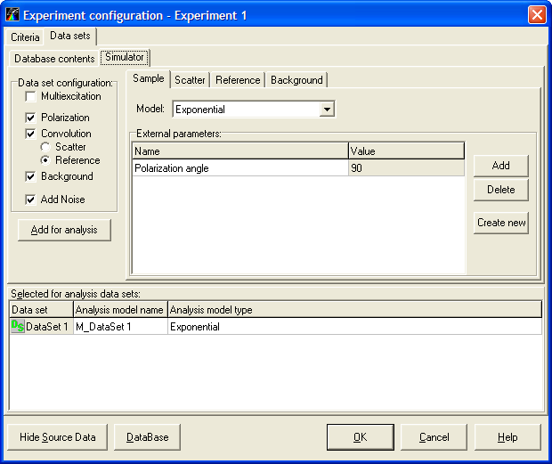
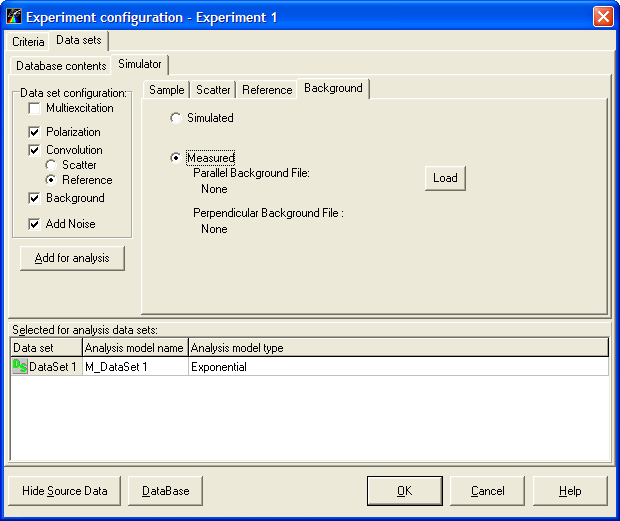
Experiment configuration window
This window is used to change the configuration of the current experiment. It provides the ability to select target fit criterion, to choose additional fit quality criteria for judging the fit results, to add and remove the data sets within the experiment and select the model that will be employed to analyze the data from the given data set.

The Experiment configuration window contains the following pages:

Criteria page allows to choose target fit criterion and select additional fit quality criteria for current experiment.

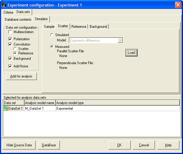
Data sets page is used for managing data sets and selecting the associated models. This page contains two subpages:
- Database contents subpage provides access to the measured data sets located in the Measurements Database.
- Simulator subpage allows to cunstruct simulation data sets and add them to the current experiment.

Note: To choose the necessary page while working with TRFA Data Processor Advanced you should click on the corresponding Tab.

An example view of the Experiment configuration window is given below:

To find out more about the functionality of any component, click this component on the figure.

Experiment configuration window
This window is used to change the configuration of the current experiment. It provides the ability to select target fit criterion, to choose additional fit quality criteria for judging the fit results, to add and remove the data sets within the experiment and select the model that will be employed to analyze the data from the given data set.

The Experiment configuration window contains the following pages:

Criteria page allows to choose target fit criterion and select additional fit quality criteria for current experiment.

Criteria page allows to choose target fit criterion and select additional fit quality criteria for current experiment.

Criteria page allows to choose target fit criterion and select additional fit quality criteria for current experiment.

Criteria page allows to choose target fit criterion and select additional fit quality criteria for current experiment.

Criteria page allows to choose target fit criterion and select additional fit quality criteria for current experiment.

To find out more about the functionality of any component, click this component on the figure.

Target optimization criterion combobox list
This combobox list is used to choose target fit criterion type.

Available fit quality criteria list
This list box contains the types of fit quality criteria currently available for judging the quality of the fit in TRFA Data Processor Advanced. In order to use any of these criteria in the current experiment one should move them to the Criteria to be used list.

Button "Add fit quality criteria"
This button moves fit quality criteria currently selected in Available fit quality criteria list to the Criteria to be used list. Fit quality criteria moved to the Criteria to be used list will be applied to judge the quality of the fit in the current experiment.

Button "Remove fit quality criteria"
This button moves the fit quality criteria currently selected in 'criteria to be used' list back to the Available fit quality criteria list thus removing them from the current experiment.

Fit quality criteria to be used list
This list box contains the types of fit quality criteria that are selected to be used in the current experiment for judging the quality of the fit. In order to exclude any of these criteria from being used in the current experiment one should move them back to the Available fit quality criteria list.

Alias
Shows the alias associated with Measurements Database.

Group combobox list
This combobox list is used to select the group of data sets that is displayed in the Data sets table. In the case if value of Group combobox list is set to All then all data sets located in the currently connected Measurements Database are displayed.

Button "Filter"
This button is used for filtering data in the Data sets table. After this button is pressed, Filter.hlp>mainFilter dialog box will be displayed. This dialog box is used for creating and applying the filter to the Data sets table.

Button "Search"
This button displays a search box for the Data sets table. If you want to find quickly the necessary item you should type the first few characters of its name and press Enter. In this case the application will automatically select for you the first item that has the name with this few characters at the beginning. To close the search box press key Esc.

Data sets table
The Data sets table displays data sets available from the Measurements Database.

To add measured data to the current experiment double click left mouse button on the data set. The Data Set with the same name will be added to the Selected for analysis data sets table.

Observations table
The Observations table displays information about observation data that belong to the data set selected in the Data sets table. Each observation represents the data (sample decay, Instrumental response function, reference compound or background) obtained in a single measurement.

Multiexcitation checkbox
If Multiexcitation checkbox is checked the sumulation data set will be configured to generate multiexcitation decays. Number of exitation pulses in such decay can be set by Pulses Count property of the simulated instrumental response function.

Polarization checkbox
If Polarization checkbox is checked the simulation data set will be configured to generate parallel and perpendicular fluorescence decays. Otherwise simulation data set will be configured to generate single fluorescence decay that corresponds to the measurement at the magic angle (54.7 degrees).

Convolution checkbox
If Convolution checkbox is checked the simulation data set will be configured to generate the sample fluorescence decay as a result of convolution of either Instrumental response function or reference compound with the decay generated by the selected model. Otherwise the convolution procedure is not performed and sample fluorescence decay is represented by an impulse response function generated by model.

Scatter radiobutton
If Scatter radiobutton is selected the simulation data set will be configured to generate the convoluted sample fluorescence decay and Instrumental response function. This radiobutton is enabled only in the case when Convolution checkbox is checked.

Reference radiobutton
If Reference radiobutton is selected the simulation data set will be configured to generate the convoluted sample fluorescence decay and reference compound. This radiobutton is enabled only in the case when Convolution checkbox is checked.

Background checkbox
If Background checkbox is checked the simulation data set will be configured to generate the background . In this case the background also will be added to the sample fluorescence decay.

Add noise checkbox
If Add noise checkbox is checked the statistical noise will be added to all simulated curves stored in the simulation data set.

Button "Add for analysis"
This button is used to add new simulation data set to the current experiment. Configuration of this simulation data set is defined by the interface elements located on the Simulator subpage of Experiment configuration window.

Model combobox list
This combobox list is used to select the model that will be used to generate the sample fluorescence decay in simulation data set.

External parameters table
The External parameters table displays and allows to change the names and values of external parameters that will be added to the simulation data set.

Button "Add external parameter"
This button adds empty external parameter to the current simulation Data Set which must be filled in. This new external parameter is displayed as a new record in the External parameters table.

Button "Delete external parameter"
This button deletes the external parameters selected in the External parameters table.

Button "Create new external parameter"
This button opens TRFAMDBAdv.hlpExternal parameters form.

Simulated radiobutton (Scatter page)
If Simulated radiobutton is selected the simulation data set will be configured to generate Instrumental response function according to the model with type specified in the Model combobox on the Scatter page.

Model combobox list (Scatter page)
This combobox list is used to select the model that will be used to generate the Instrumental response function in simulation data set.

Measured radiobutton (Scatter page)
If Measured radiobutton is selected the simulation data set will be configured to use Instrumental response function loaded from Measurements Database. The data for Instrumental response function can be loaded using Load button located on the Scatter page.

Reference file/Parallel reference file label
This label shows the name of the Observation record located in Measurements Database that contains the data that will be used either as Instrumental response function (in the case data set contains data without polarization) or as parallel component of Instrumental response function (in the case data set contains polarized data).

Perpendicular scatter file label
This label shows the name of the Observation record located in Measurements Database that contains the data that will be used as perpendicular component of Instrumental response function. This label is accessible only in the case if data set contains polarized data.

Load button (Scatter page)
This button opens Select file(s) dialog box for selecting and loading files located in the Measurements Database.

Simulated radiobutton (Reference page)
If Simulated radiobutton is selected the simulation data set will be configured to use one-exponential model to generate Reference compound. The reference decay time is specified in the Life time edit on the Reference page.

Reference Life time edit
This edit allows to input the reference decay time in the case if one-exponential model is used to simulate Reference compound. This edit is enabled only if Simulated radiobutton is selected.

Measured radiobutton (Reference page)
If Measured radiobutton is selected the simulation data set will be configured to use Reference compound loaded from Measurements Database. The data for Reference compound can be loaded using Load button located on the Reference page.

Reference file/Parallel reference file label
This label shows the name of the Observation record located in Measurements Database that contains the data that will be used either as Reference compound (in the case data set contains data without polarization) or as parallel component of Reference compound (in the case data set contains polarized data).

Perpendicular reference file label
This label shows the name of the Observation record located in Measurements Database that contains the data that will be used as perpendicular component of Reference compound. This label is accessible only in the case if data set contains polarized data.

Load button (Reference page)
This button opens Select file(s) dialog box for selecting and loading files located in the Measurements Database.

Simulated radiobutton (Background page)
If Simulated radiobutton is selected the simulation data set will be configured to generate time-independent background noise and add it to the sample decay. The level of this noise is specified using the Level property of the Background object.

Measured radiobutton (Background page)
If Measured radiobutton is selected the simulation data set will be configured to use Background loaded from Measurements Database. The data for Background can be loaded using Load button located on the Background page.

Background file/Parallel background file label
This label shows the name of the Observation record located in Measurements Database that contains the data that will be used either as Background (in the case data set contains data without polarization) or as parallel component of Background (in the case data set contains polarized data).

Perpendicular background file label
This label shows the name of the Observation record located in Measurements Database that contains the data that will be used as perpendicular component of Background. This label is accessible only in the case if data set contains polarized data.

Load button (Background page)
This button opens Select file(s) dialog box for selecting and loading files located in the Measurements Database.

Selected for analysis data sets table
Local menu

Selected for analysis data sets table is used for displaying Data Sets within the experiment and the models, that correspond to them.
This Table contains the following columns:
? Data set displays the names of the Data Sets contained in the current experiment (The values in this column can be changed only for Simulation Data Sets).
? Analysis model name displays the name of the analysis model related to the current Data Set.
? Analysis model type displays the analysis model type.

Button "Hide/Show Source Data"
This button hides/shows Database contents page and Simulator page.

Button "DataBase"
This button opens Measurements Database. You can use this Database as more advanced way to navigate through your data and add some of them to the current experiment for analysis.

Button "Ok"
This button finishes work with the Experiment configuration window and applies all configuration changes to the current experiment.

Button "Cancel"
This button finishes work with the Experiment configuration window without changing the configuration of the current experiment.

Button "Help"
This button opens the help window that describes how to work with Experiment Configuration window.

Export data dialog box
This dialog box is used to export the target criterion value, fit quality criteria values, parameter groups, free parameters and arrays of decays, residuals and residuals autocorrelation to the text file.

An example view of the Export data dialog box is given below:

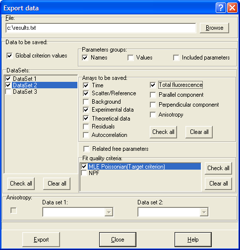
To find out more about the functionality of any component, click this component on the figure.

"File" edit
This box contains the name of the file where experiment data will be exported.

Button "Browse"
This button displays the standard Open dialog box in which the path and the name of the file can be chosen.

"Global criterion values" check box
If this check box is checked, the target fit criterion values will be exported.

"Parameters groups" group box
This group box provides a possibility to export the data related to parameters groups.
The following information about the parameters groups can be exported:
? Names
? Values
? Included parameters

"Data Sets" group box
This group box is used to choose the Data Sets, the data will be exported from.

Data sets list contains the names of the available data sets.
Button {bmc BtnCheckAll.bmp} selects all data sets.
Button {bmc BtnClearAll.bmp} unselects all data sets.

"Arrays to be saved" group box
This group box is used to choose the arrays of values to be saved. Check the corresponding check box to export the certain array.
The following arrays of values are available for the export:
? Time -- the time scale points at which decays are calculated
? Scatter/Reference -- the data for Instrumental response function or Reference decay
? Background -- the data for Background
? Experimental data -- measured or simulated sample decay data
? Theoretical data -- the data for decay calculated with chosen theoretical model
? Residuals
? Autocorrelation -- residuals autocorrelation data

? Total fluorescence -- selects for the export the arrays related to the total fluorescence decay
? Parallel component -- selects for the export the arrays related to the parallel fluorescence decay component
? Perpendicular component -- selects for the export the arrays related to the perpendicular fluorescence decay component
? Perpendicular component -- selects for the export the arrays related to the perpendicular fluorescence decay component. This option is used to export anisotropy decay calculated from parallel and perpendicular polarization components that are located in one data set.

Button {bmc BtnCheckAll.bmp} selects all arrays.
Button {bmc BtnClearAll.bmp} unselects all arrays.

"Related free parameters" check box
If this check box is checked, the information about unlinked parameters related to each data set selected in the Data Sets list will be exported.

"Fit quality criteria" group box
This group box is used to choose the Fit quality ctiteria that should be exported.

Fit quality criteria list contains the names of the available fit quality criteria.
Button {bmc BtnCheckAll.bmp} selects all fit quality criteria.
Button {bmc BtnClearAll.bmp} unselects all fit quality criteria.

"Anisotropy" group box
This group box is used to export arrays related to the anisotropy decay calculated from polarization components (for example, parallel and perpendicular) that are located in two different data sets. It is supposed that these data sets were analyzed globally with anisotropy model.

The Anisotropy group box contains the following components:
Check box that should be checked to export arrays related to the anisotropy decay.
Data set 1 combobox is used to select first data set for calculating anisotropy decay.
Data set 2 combobox is used to select second data set for calculating anisotropy decay.

Button "Export"
This button executes the export procedure.

Button "Close"
This button finishes work with Export data dialog box.

Button "Help"
This button opens the help window that describes how to work with Export data dialog box.

Select file(s) dialog box
This dialog box is used to load data from observation records located in the Measurements Database. These data can be used by the built-in simulator as Instrumental response function, Reference compound or Background. In the case if simulation data set is supposed to contain polarization components (Polarization checkbox in Experiment configuration window is checked) then Select files(s) dialog box allows to choose data for parallel and perpendicular components of corresponding curve simultaneously.

An example view of the Select files(s) dialog box is given below:

To find out more about the functionality of any component, click this component on the figure.

Button "Sort ascending"
This button sorts the records in the Files table by the "File name" field in the ascending order.

Button "Sort descending"
This button sorts the records in the Files table by the "File name" field in the descending order.

Button "Search"
This button displays a search box for the Files table. If you want to find quickly the necessary item you should type the first few characters of its name and press Enter. In this case the application will automatically select for you the first item that has the name with this few characters at the beginning. To close the search box press key Esc.

Button "Filter"
This button is used for filtering data in the Files table. After this button is pressed, Filter.hlp>mainFilter dialog box will be displayed. This dialog box is used for creating and applying the filter to the Files table.

Files table
The Files table displays observations available from the Measurements Database for the curve (Instrumental response function, Reference compound or Background) with corresponding type and polarization.

Button "Ok"
This button finishes work with the Select files(s) dialog box and chooses file(s) currently selected in the Files table to be used in the built-in simulator.

Button "Cancel"
This button finishes work with the Select files(s) dialog box without changing the settings of the built-in simulator.

Button "Help"
This button opens the help window that describes how to work with Select files(s) dialog box.

Load and apply an existing template dialog box
This dialog box is used to load and apply a previously saved template.
An example view of the Load and apply an existing template dialog box is given below:

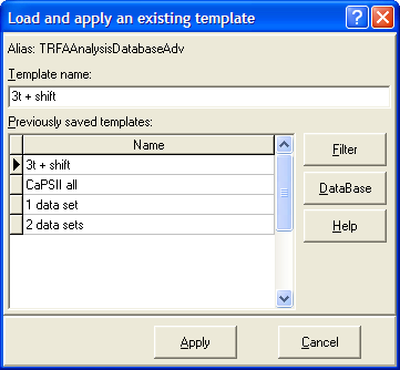
To find out more about the functionality of any component, click this component on the figure.

Alias label
Shows the alias associated with Templates Database.

Template name edit
Is used for entering the name of the template you want to load from the Templates Database.
You can quickly find the template you want to load by typing the first few characters of its name. In this case the application will automatically select for you the first template that has the name with this few characters at the beginning.

Previously saved templates list
This list displays the templates previously saved in the Templates Database. If the filter is applied, the currently displayed template names depend on the filter criteria.

Button "Filter"
This button opens Filter.hlp>mainFilter dialog box, that allows to create the filter that can be applied to the Previously saved templates list. If this filter is applied, the only template names that correspond to the filter criteria will be displayed.

Button "DataBase"
This button opens Templates Database and sets the record selected in the Load and apply an existing template dialog box as the current record.

Button "Help"
This button opens the help window that describes how to work with Load and apply an existing template dialog box.

Button "Apply"
This loads and applies the selected template. After pressing this button the progress bar window appears. This progress bar window contains a number progress bars for displaying the progress of the template loading procedure.

Button "Cancel"
This button finishes work with the dialog box without loading and applying any templates.

Create and save new template dialog box
This dialog box is used to create and save a new template.
An example view of the Create and save new template dialog box is given below:

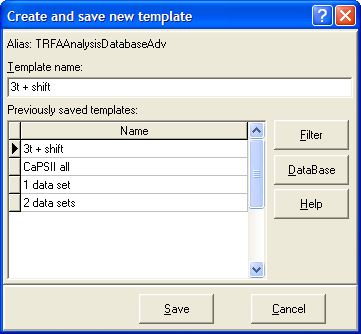
To find out more about the functionality of any component, click this component on the figure.

Alias label
Shows the alias associated with Templates Database.

Template name edit
This edit is used for entering the name for the template you are creating and saving.

Previously saved templates list
This list displays the templates previously saved in the Templates Database. If the filter is applied, the currently displayed template names depend on the filter criteria.

Button "Filter"
This button opens Filter.hlp>mainFilter dialog box, that allows to create the filter that can be applied to the Previously saved templates list. If this filter is applied, the only template names that correspond to the filter criteria will be displayed.

Button "DataBase"
This button opens Templates Database and sets the record selected in the Create and save new template dialog box as the current record.

Button "Help"
This button opens the help window that describes how to work with Create and save new template dialog box.

Button "Save"
This button creates and saves the new template using selected name.

Button "Cancel"
This button finishes work with the dialog box without creating and saving current template.

"Fit parameter vs. external parameter view" window
This window displays the dependence of the value of the given fit parameter on the external parameter.
An example of the "Fit parameter vs. external parameter view" window is given on the following figure:

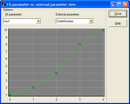
To find out more about the functionality of any component, click this component on the figure.

Fit parameter combobox list
This combobox list is used to chose fit parameter to be displayed on the graph.

External parameter combobox list
This combobox list is used to chose external parameter.

2D Chart
This 2D Chart displays the Fit parameter vs. external parameter curve. The values of the fit parameter are displayed along the vertical axis and the values of the external parameter are displayed along the horizontal axis.

With 2D Chart you can:
? move curve in the box by keeping the right mouse button down and moving the mouse pointer through the box.
? zoom in the image by dragging the cursor diagonally across the necessary area from left top corner to right bottom corner.
? restore whole view of the image by pressing left mouse button and dragging mouse pointer on some positions to upper left.

Additional actions with 2D Chart available through the local menu.

Button "Close"
This button closes the "Fit parameter vs. external parameter view" window.

Button "Help"
This button opens the help window that describes how to work with "Fit parameter vs. external parameter view" window.

Anisotropy view window
This window displays measured (green) and theoretical (red) anisotropy decays, weighted residuals and residuals autocorrelation function. Anisotropy decays are calculated from polarization components (for example, parallel and perpendicular) that are located in two different data sets. The theoretical anisotropy decays, weighted residuals and residuals autocorrelation function are displayed only in the case if data sets within current experiment were analyzed.

An example of the Anisotropy view window is given on the following figure:

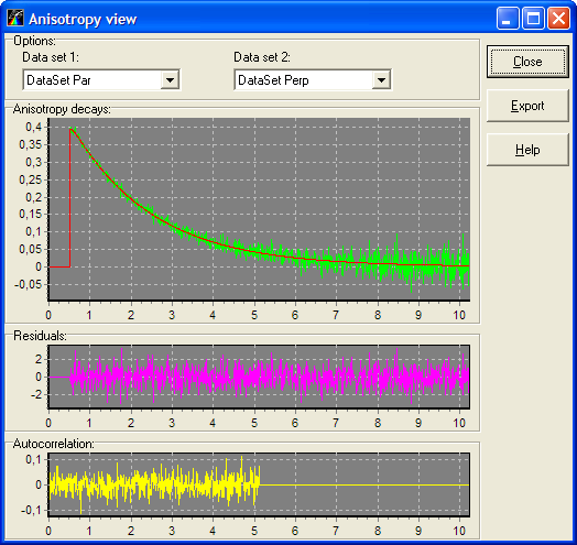
To find out more about the functionality of any component, click this component on the figure.

Options group box
The elements of this group box are used to select the pair of data sets required to calculate the anisotropy decays.

The Anisotropy group box contains the following components:
Data set 1 combobox is used to select first data set for calculating anisotropy decay.
Data set 2 combobox is used to select second data set for calculating anisotropy decay.

Anisotropy decays chart
This 2D Chart displays the measured and theoretical anisotropy decays. By default measured anisotropy decay is green and theoretical anisotropy decay is red.

With 2D Chart you can:
? move curve in the box by keeping the right mouse button down and moving the mouse pointer through the box.
? zoom in the image by dragging the cursor diagonally across the necessary area from left top corner to right bottom corner.
? restore whole view of the image by pressing left mouse button and dragging mouse pointer on some positions to upper left.

Additional actions with 2D Chart available through the local menu.

Residuals chart
This 2D Chart displays the weighted residuals calculated from measured and theoretical anisotropy decays. The expression that is applied to calculate weighted residuals depends on the type of target fit criterion that is used in the current experiment.

With 2D Chart you can:
? move curve in the box by keeping the right mouse button down and moving the mouse pointer through the box.
? zoom in the image by dragging the cursor diagonally across the necessary area from left top corner to right bottom corner.
? restore whole view of the image by pressing left mouse button and dragging mouse pointer on some positions to upper left.

Additional actions with 2D Chart available through the local menu.

Residuals autocorrelation chart
This 2D Chart displays the autocorrelation function of weighted residuals.

With 2D Chart you can:
? move curve in the box by keeping the right mouse button down and moving the mouse pointer through the box.
? zoom in the image by dragging the cursor diagonally across the necessary area from left top corner to right bottom corner.
? restore whole view of the image by pressing left mouse button and dragging mouse pointer on some positions to upper left.

Additional actions with 2D Chart available through the local menu.

Button "Close"
This button closes the Anisotropy view window.

Button "Export"
This button is used to export the arrays of anisotropy decays, residuals and residuals autocorrelation to the text file.

Button "Help"
This button opens the help window that describes how to work with Anisotropy view window.

Add/Remove constraints dialog box
This dialog box is used to manage functional constraints associated with the current model. The Add/Remove constraints dialog box can be accessed via Constraints property of the model.
An example view of the Add/Remove constraints dialog box is given below:

To find out more about the functionality of any component, click this component on the figure.

Available constraints list
This list box contains the types of functional constraints currently available for associating with the model in TRFA Data Processor Advanced. In order to associate any of these constraints with the current model one should copy its name to the corresponding Created constraints list. In the case if several functional constraints of the same type should be created for the current model the name of the corresponding constraint should be copied to the Created constraints list several times.

Created constraints list
This list box contains the types of functional constraints that are created for the current model and can be used to limit the change of the fit parameter values during the fit. In order to exclude any of these constraints from being used in the current model one should select them and remove using Remove constraint button.

Button "Add constraint"
This button creates new functional constraint with type currently selected in the Available constraints list and adds it to the Created constraints list of the current model.

Button "Remove constraint"
This button removes the constraint currently selected in Created constraints list.

Button "Configure"
This button opens the configuration dialog box for the constraint currently selected in the Created constraints list.

Button "Ok"
This button finishes work with the Add/Remove constraints dialog box and applies all changes in the constraint lists to the current model.

Button "Cancel"
This button finishes work with the Add/Remove constraints dialog box without changing the list of constraints associated with the current model.

Button "Help"
This button opens the help window that describes how to work with Add/Remove constraints dialog box.

Ratio constraint configuration dialog box
This dialog box is used to configure Ratio constraint.
An example view of the Ratio constraint configuration dialog box is given below:

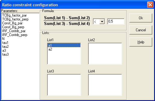
To find out more about the functionality of any component, click this component on the figure.

Parameters list
This list box contains the list of model parameters that can be used in the Ratio constraint formula. In order to include any parameter to the constraint formula one should select this parameter and drag it to one of the list boxes that belong to the Lists group box.

Sign combobox
This combobox allows to select the sign ('<' or '>') that is used to compare the left and right side of the Ratio constraint formula.

Right side value edit
This edit allows to put in the numerical value that is used as right side of the Ratio constraint formula.

Lists groupbox
This groupbox contains four listboxes that are used for storing the parameters that should be included to the corresponding parameter groups in the Ratio constraint formula. In order to add any fit parameter to one of the lists that belong to Lists groupbox one should select this parameter in the
Parameters list and drag it to the corresponding list. In order to remove the fit parameter from one of the lists that belong to Lists groupbox one should select this parameter and drag it back to the Parameters list.

Button "Ok"
This button finishes work with the Ratio constraint configuration dialog box and applies all changes to the Ratio constraint.

Button "Cancel"
This button finishes work with the Ratio constraint configuration dialog box without changing the settings of the Ratio constraint.

Button "Help"
This button opens the help window that describes how to work with Ratio constraint configuration dialog box.

Associations window
This window is used to manage associations between exponential terms that describe total fluorescence decay and anisotropy decay in the anisotropy model equation.
An example view of the Associations window is given below:

To find out more about the functionality of any component, click this component on the figure.

Associations table
This table allows to set and remove associations between exponential terms that describe total fluorescence decay and anisotropy decay. The columns and rows of the associations table correspond to the separate exponents that describe, respectively, total fluorescence decay and anisotropy decay. In order to set association between certain fluorescence and anisotropy exponents the checkbox located in corresponding table cell should be checked. In the case if certain association should be removed the corresponding checkbox should be unchecked.

Button "Check all"
This button checks all checkboxes in the associations table.

Button "Clear all"
This button unchecks all checkboxes in the associations table.

Button "Ok"
This button finishes work with the Associations window and applies all changes to the current anisotropy model.

Button "Cancel"
This button finishes work with the Associations window without changing the settings of the anisotropy model.

Button "Help"
This button opens the help window that describes how to work with Associations window.

Multi-exponential model
In a variety of applications, fluorescence decay of the sample and the sample anisotropy decay can be adequately approximated by a sum of exponentials [1-3]. The form of the equations that underlie the multi-exponential model depends on the model settings.
By default (the property FluorParametersType is set to "Amplitudes and decay times") the multi-exponential model uses the following equation to calculate the impulse response function of the sample I(t):

(1)

where

and

(j=1,...,M) are, respectively, the amplitudes and decay times of corresponding exponents; M is the number of exponents in the sum.
Sometimes instead of amplitudes

it is more convenient to use contributions of exponents (the property FluorParametersType is set to "Contributions and decay times"). The sum of contributions is always equal to 1. Therefore such coefficients being multiplied on 100 show the contribution of each exponent in the sum expressed as percentage. Since in some cases the negative pre-exponential multipliers are required to describe the sample fluorescence decay (for example, in the case if impulse response function of the sample I(t) rises at the beginning) the equations for I(t) can contain some exponents with pre-exponential factors less than 0. Switching between amplitudes and contributions is controlled by Normalization property of multi-exponential model and can be done independently for positive and negative pre-exponential factors. Therefore in the case if contributions are used I(t) is calculated as follows:
1. The value of Normalization property is set to Positive:

(2)
2. The value of Normalization property is set to Negative:

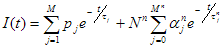
(3)
3. The value of Normalization property is set to Positive and Negative:

(4)

where

(j=1,...,M) are contributions of corresponding exponents with positive pre-exponential factors; N is normalization parameter for exponents with positive pre-exponential factors;

and

(j=0,...,

) are respectively amplitudes, contributions and decay times of corresponding exponents with negative pre-exponential factors;

is normalization parameter for exponents with negative pre-exponential factors;

is a number of exponents with negative pre-exponential factors.
Besides the equations (1) and (2) the multi-exponential model can calculate impulse response function of the sample I(t) using the equation that contains the ratio of amplitudes (the property FluorParametersType is set to "Ratio and decay times"). This equation has the form:

(5)
where

(j=2,...,M) are the ratios of amplitudes of corresponding exponents to the amplitude of first exponent.

In the case if multi-exponential model is used to perform the two stage anisotropy analysis it can also calculate the theoretical anisotropy decay as follows:

(6)
where

and

(j=1,...,K) are, respectively, the amplitudes and rotational correlation times of corresponding exponents; K is the number of exponents in the sum.

Multi-exponential model properties:
1. Properties common for all models;
2. Fluor IG type determines how the initial guesses for parameters in eq. 1-5 are generated;
3. FluorParametersType defines the form of equation (see eq. 1-5 above) that is used to generate the impulse response function of the sample I(t);
4. FluorExponentsCount defines the number of exponents in eq. 1 and 5 shown above. This property is available only in the case if FluorParametersType property is set either to Amplitudes and decay times or to Ratio and decay times;
5. PosFluorExponentsCount defines the number of exponents with positive pre-exponential factors in eq. 3-4 shown above. This property is available only in the case if FluorParametersType property is set to Contributions and decay times;
6. Anis IG type determines how the initial guesses for parameters in eq. 6 are generated. This property is available only in the case if Analysis type property of Experiment object is set to Anisotropy;
7. AnisExponentsCount defines the number of exponents in eq. 6 shown above. This property is available only in the case if Analysis type property of Experiment object is set to Anisotropy;
8. NegFluorExponentsCount defines the number of exponents with negative pre-exponential factors in eq. 3-4 shown above. This property is available only in the case if FluorParametersType property is set to Contributions and decay times;
9. Normalization selects the type of positive and negative pre-exponential factors (amplitudes or contributions) that are used by multi-exponential model and chooses one of the formulas 2-4 for calculating I(t). This property is available only in the case if FluorParametersType property is set to Contributions and decay times.

Multi-exponential model parameters:
1. Parameters common for all models;
2. pi is the amplitude of the i-th exponent in the eq. 1 and 3. This parameter is available either in the case if FluorParametersType property is set either to Amplitudes and decay times or if FluorParametersType property is set either to Contributions and decay times and Normalization property is set to Negative;
3. ai is the contribution of the i-th positive exponent. This parameter is available only in the case if FluorParametersType property is set to Contributions and decay times and Normalization property is set either to Positive or to Positive and Negative;
4. ri is the ratio of the (i+1)-th exponent amplitude to the amplitude of the first exponent. This parameter is available only in the case if FluorParametersType property is set either to Ratio and decay times;
5. N is the is normalization parameter for exponents with positive pre-exponential factors. This parameter is available either in the case if FluorParametersType property is set to Ratio and decay times or FluorParametersType property is set to Contributions and decay times and Normalization property is set either to Positive or to Positive and Negative;
6. a_ni is the contribution of the i-th negative exponent. This parameter is available only in the case if FluorParametersType property is set to Contributions and decay times and Normalization property is set either to Negative or to Positive and Negative;
7. N_n is the is normalization parameter for exponents with negative pre-exponential factors. This parameter is available only in the case if FluorParametersType property is set to Contributions and decay times and Normalization property is set either to Negative or to Positive and Negative;
8. taui is the decay time of the i-th exponent in eq. 1, 5 and the decay time of the i-th exponent with positive pre-exponential factor in eq. 2-4;
9. tau_ni is the decay time of the i-th exponent with negative pre-exponential factor. This parameter is available only in the case if FluorParametersType property is set to Contributions and decay times;
10. betai is the amplitude of the i-th exponent in the eq. 6 for anisotropy decay. This parameter is available only in the case if Analysis type property of Experiment object is set to Anisotropy;
11. phii is the rotational correlation time of the i-th exponent in the eq. 6 for anisotropy decay. This parameter is available only in the case if Analysis type property of Experiment object is set to Anisotropy.

External parameters required by multi-exponential model:
This model does not require any external parameters.

Analysis types supported by multi-exponential model:
1. Analysis of single fluorescence decay;
2. Global analysis;
3. Two stage anisotropy analysis.

Anisotropy model
The anisotropy model is implemented in TRFA Data Processor Advanced to provide the anisotropy analysis based on the global fit. The model generates the impulse response function of the sample I(t) according to the following equation:

where A is the normalization parameter;

and

(i=1,...,M) are, respectively, contributions and decay times of corresponding fluorescence exponents;

is the polarization angle;

is the anisotropy decay level under the assumption that

;

coefficient that is equal to 1 if i-th fluorescence and j-th anisotropy exponents are associated, otherwise

is 0;

and

(j=1,...,K) are, respectively, the amplitudes and rotational correlation times of corresponding anisotropy exponents.
The anisotropy model can be configured to perform non-associative and associative anisotropy analysis. The type of anisotropy analysis can be defined by setting the coefficients

(see eq. above). The coefficients

can be managed using Associations window that is displayed using the Associations property of the anisotropy model. By default the anosotropy model is configured for non-associative anisotropy analysis (all coefficients

are set to 1). In the case if associative anisotropy analysis should be done (only certain associations between fluorescence and anisotropy exponents exist) the coefficients

that correspond to the unnecessary associations should be set to 0.

Anisotropy model properties:
1. Properties common for all models;
2. Fluor IG type determines how the initial guesses for parameters are generated;
3. FluorExponentsCount defines the number M of fluorescence exponents in equation shown above;
4. AnisExponentsCount defines the number K of anisotropy exponents in equation shown above;
5. Associations displays Associations window that allows managing the associations between fluorescence and anisotropy exponents.

Anisotropy model parameters:
1. Parameters common for all models;
2. A is the normalization parameter;
3. alphai is the contribution of the i-th fluorescence exponent;
4. taui is the decay time of the i-th fluorescence exponent;
5. r_inf is the anisotropy decay level under the assumption that

;
6. betaj is the amplitude of the j-th anisotropy exponent;
7. phij is the rotational correlation time of the j-th anisotropy exponent.

External parameters required by anisotropy model:
1. Polarization angle defines the angle of polarizer orientation in degrees that corresponds to the data associated with the anisotropy model.

Analysis types supported by anisotropy model:
1. Anisotropy analysis based on the global fit.

Gauss distribution of decay rates model
The gauss distribution of decay rates model [4, 5] generates the impulse response function of the sample I(t) according to the following formula:

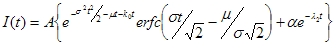
where A is the normalization parameter; s is the standard deviation on decay rate; m is average decay rate; k0 denotes the minimum decay rate; erfc denotes the complementary error function; a defines the relative contribution of second fluorescence component; l2 is the inverted decay time of second fluorescence component.

Gauss distribution of decay rates model properties:
1. Properties common for all models;
2. Fluor IG type determines how the initial guesses for parameters are generated.

Gauss distribution of decay rates model parameters:
1. Parameters common for all models;
2. A is the normalization parameter;
3. sigma is standard deviation on decay rate;
4. mu is average decay rate;
5. k0 is minimum decay rate;
6. alpha defines the relative contribution of second fluorescence component;
7. lambda2 is inverted decay time of second fluorescence component.

External parameters required by gauss distribution of decay rates model:
This model does not require any external parameters.

Analysis types supported by gauss distribution of decay rates model:
1. Analysis of single fluorescence decay;
2. Global analysis.

Poisson distribution of decay rates model
The Poisson distribution of decay rates model [6, 7] generates the impulse response function of the sample I(t) according to the following formula:

where A is the normalization parameter; l1 is the inverted decay time of first fluorescence component in absence of energy transfer or other quenching; c is concentration; b1 is quenching efficiency of first fluorescence component; m is average number of quenchers; e is the rate of quenching for a probe interacting with one quencher; a defines the relative contribution of second fluorescence component; l2 is the inverted decay time of second fluorescence component in absence of energy transfer or other quenching.

Poisson distribution of decay rates model properties:
1. Properties common for all models;
2. Fluor IG type determines how the initial guesses for parameters are generated.

Poisson distribution of decay rates model parameters:
1. Parameters common for all models;
2. A is the normalization parameter;
3. lambda1 is the inverted decay time of first fluorescence component in absence of energy transfer or other quenching;
4. beta1 is quenching efficiency of first fluorescence component;
5. mu is average number of quenchers;
6. epsilon is rate of quenching for a probe interacting with one quencher;
7. alpha defines the relative contribution of second fluorescence component;
8. lambda2 is inverted decay time of second fluorescence component in absence of energy transfer or other quenching.

External parameters required by Poisson distribution of decay rates model:
1. Concentration defines the concentration

Analysis types supported by Poisson distribution of decay rates model:
1. Analysis of single fluorescence decay;
2. Global analysis.

2 - compartmental model
The 2-compartmental model [8, 9] is designed to describe the behavior of a dynamic, linear, time-invariant, intermolecular system consisting of two distinct types of ground-state species and two corresponding excited-state species. This system can be presented by the following scheme:

As it is shown on the scheme above ground-state species 1 can reversibly react with co-reactant M to form ground-state species 2. Excitation by light creates the excited-state species 1* and 2*, which can decay by fluorescence (F) and non-radiative (NR) processes. The composite rate constant for these processes is denoted by k0i (= kFi + kNRi) for species i* (i=1,2). k21 represents the second-order rate constant for the association 1* + M ® 2*, while k12 is the first-order rate constant for dissociation of 2* into 1* and M.
The impulse response function of the sample I(t) for the system described above can be calculated according to the following equation:

where D is the proportionality coefficient; C is the 1 ? 2 vector that contains the emission weighting factors of species 1* and 2* at emission wavelength; B is the 2 x 1 vector whose elements represent the concentration of species 1* and 2* at time zero. A is 2 x 2 matrix defined as follows:

where k01, k02, k12, k21 are the rate constants described above; [M] is the co-reactant concentration.

2-compartmental model properties:
1. Properties common for all models;
2. Fluor IG type determines how the initial guesses for parameters are generated.

2-compartmental model parameters:
1. Parameters common for all models;
2. D is the normalization parameter;
3. C1 is the emission weighting factor of species 1*;
4. C2 is the emission weighting factor of species 2*;
5. K01 is the composite rate constant of species 1*;
6. K12 is the first-order rate constant for dissociation of 2* into 1* and co-reactant M;
7. K21 represents the second-order rate constant for the association 1* + M ® 2*;
8. K02 is the composite rate constant of species 2*;
9. B1 is the concentration of species 1* at time zero;
10. B2 is the concentration of species 2* at time zero.

External parameters required by 2-compartmental model:
1. [M] is the co-reactant concentration.

Analysis types supported by 2-compartmental model:
1. Analysis of single fluorescence decay;
2. Global analysis.

3 - compartmental model
The 3-compartmental model [10-12] is designed to describe the behavior of a causal, linear, time-invariant, intermolecular system consisting of three distinct types of ground-state species (1, 2, 3) and three corresponding excited-state species (1*, 2*, 3*). This system can be presented by the following scheme:

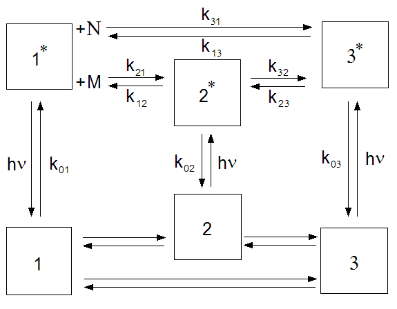
As it is shown on the scheme above species 1 (respectively 1*) can reversibly react with co-reactant M to form species 2 (respectively 2*). Also species 1 (respectively 1*) can reversibly react with co-reactant N to form species 3 (respectively 3*). Also the excited-state interconversion between states 2* and 3* exists. The excited-state species 1*, 2* and 3* created by light excitation can decay by fluorescence (F) and non-radiative (NR) processes. The composite rate constant for these processes is denoted by k0i (= kFi + kNRi) for species i* (i=1, 2, 3). k21 and k31 represent respectively the second-order rate constants for the association 1* + M ® 2* and 1* + N ® 3*. The dissociations 2* ® 1* + M and 3* ® 1* + N are respectively characterized by first-order rate constants k12 and k13. The rate constants k23 and k32 describe the direct interconversion between species 2* and 3*.
The impulse response function of the sample I(t) for the system described above can be calculated according to the following equation:

where D is the proportionality coefficient; C is the 1 ? 3 vector that contains the emission weighting factors of species 1*, 2* and 3* at emission wavelength; B is the 3 x 1 vector whose elements represent the concentration of species 1*, 2* and 3* at time zero. A is 3 x 3 matrix defined as follows:

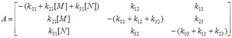
where k01, k12, k13, k21, k02, k23, k31, k32, k03, are the rate constants described above; [M] and [N] are concentrations for corresponding co-reactants.

2-compartmental model properties:
1. Properties common for all models;
2. Fluor IG type determines how the initial guesses for parameters are generated.

2-compartmental model parameters:
1. Parameters common for all models;
2. D is the normalization parameter;
3. C1 is the emission weighting factor of species 1*;
4. C2 is the emission weighting factor of species 2*;
5. C3 is the emission weighting factor of species 3*;
6. K01 is the composite rate constant of species 1*;
7. K12 is the first-order rate constant for dissociation of 2* into 1* and co-reactant M;
8. K13 is the first-order rate constant for dissociation of 3* into 1* and co-reactant N;
9. K21 represents the second-order rate constant for the association 1* + M ® 2*;
10. K02 is the composite rate constant of species 2*;
11. K23 is the interconversion rate constant from state 3* to 2*;
12. K31 represents the second-order rate constant for the association 1* + N ® 3*;
12. K32 is the interconversion rate constant from state 2* to 3*;
13. K03 is the composite rate constant of species 3*;
14. B1 is the concentration of species 1* at time zero;
15. B2 is the concentration of species 2* at time zero.
16. B3 is the concentration of species 2* at time zero.

External parameters required by 2-compartmental model:
1. [M] is the co-reactant M concentration.
2. [N] is the co-reactant N concentration.

Analysis types supported by 2-compartmental model:
1. Analysis of single fluorescence decay;
2. Global analysis.

Chi-square target fit criterion
The chi-square target fit criterion [13, 14] estimates the degree of conformity of measured (simulated) decays and theoretical decays generated by models. The equation that underlies this target fit criterion can be obtained on the basis of Maximum Likelihood method assuming Gaussian statistics of the noise in the measured (simulated) data. The value of chi-square target fit criterion is calculated by the following formula:

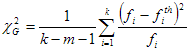
where

and

are, respectively, the values of measured (simulated) and theoretical fluorescence decays in a certain channel (in the case of global analysis

and

denote the values of all analyzed decays); k is the number of points in all decays that participate in calculation of chi-square; m is the number of fit parameters that should be estimated.
For good fit the final value of chi-square target fit criterion obtained after the analysis should be close to 1.

MLE poissonian target fit criterion
The MLE poissonian target fit criterion [15] estimates the degree of conformity of measured (simulated) decays and theoretical decays generated by models. The equation that underlies this target fit criterion can be obtained on the basis of Maximum Likelihood method assuming Poissonian statistics of the noise in the measured (simulated) data. The value of MLE poissonian target fit criterion is calculated by the following formula:

where

and

are, respectively, the values of measured (simulated) and theoretical fluorescence decays in a certain channel (in the case of global analysis

and

denote the values of all analyzed decays); k is the number of points in all decays that participate in calculation of MLE poissonian target fit criterion; m is the number of fit parameters that should be estimated.
For good fit the final value of MLE poissonian target fit criterion obtained after the analysis should be close to 1.

Standard normal deviation Zc2
Since the value of target fit criterion (c2) is dependent on the number of degrees of freedom in the data, it is possible to calculate the normal deviation Zc2 by the following equation [17, 18]:

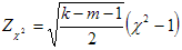
where k is the number of points in all decays that participate in calculation of c2; m is the number of fit parameters that should be estimated. The value Zc2 is normally distributed, so that the tables for normal distribution can be used to judge the quality of the fit at certain confidence level. Thus |Zc2|<1.96 for testing at confidence level 95%; |Zc2|<2.58 (99%) and |Zc2|<3.3 (99,9%).

Durbin-Watson parameter
The Durbin-Watson parameter d is used to test for serial correlation between residuals and can be calculated by the following formula [18, 19]:

where Ri is the value of the residual in the i-th point; k is the number of points where residuals are calculated. To make decision about the quality of the fit the calculated Durbin-Watson parameter value should be compared with the values dL and dU (lesser and upper values). These values can be taken from corresponding tables and depend on the number of points k (see equation above) and on the numbers of independent variables. If d<dL the residuals are correlated. In the case if d>dU the residuals are regarded as uncorrelated. When dL < d < dU no conclusions about correlation of residuals can be made.

Runs test
The ordinary runs test [20] is applied to check the randomness of the residuals signs versus channel number. In this test the actual number of ordinary runs R is calculated and compared with expected number Rexp. The term ordinary run denotes the consecutive sequence of residuals with the same sign. If the sequence of residuals is random the expected number of runs Rexp and number of runs variance

are calculated as follows:

where P and N are respectively the number of residuals with positive and negative sign. The values defined above enable to calculate the runs test parameter Z that will be distributed approximately as a standard normal deviate:

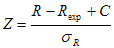
where C is the continuity correction which partially compensates for the approximation of a discrete distribution by a continuous distribution. The value of C depends on the number of tested runs R. In the case if R is low (R < Rexp) C = 0.5. Otherwise (R > Rexp) C = -0.5. The calculated value Z can be used to make decision about the randomness of the residuals. The value |Z| should be compared at the certain confidence level with the value taken from tables for normal distribution. Thus |Z|<1.96 for testing at confidence level 95%. The greater the value of |Z|, the greater the probability that some correlation exists in the residuals.

Weighted residuals
The graphical dependence of weighted residuals on time channel is calculated to provide visual estimation of conformity between measured (simulated) decays and theoretical decays generated by models. The equation that is used for calculation of weighted residuals depends on the type of target fit criterion that is applied for the analysis.
In the case if chi-square target fit criterion is used for the fit the weighted residuals in i-th channel Ri are calculated by the following equation:

where

and

are, respectively, the values of measured (simulated) and theoretical fluorescence decays in i-th channel.
In the case if MLE poissonian target fit criterion is used for the fit the weighted residuals in i-th channel Ri are calculated by the following equation:

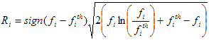
where function sign(x) is equal to 1 in the case if x is positive and -1 in the case if x is negative.

For successful fits the resuduals should be randomly distributed around 0.

Autocorrelation function of the residuals
The plot of residuals autocorrelation function [1, 17] against the time channel provides the useful visual check of the quality of the fit. The autocorrelation function shows the correlation between the residuals that are certain channels apart. The autocorrelation function of weighted residuals in the j-th channel Cj (j = 1,...,m) is calculated by the following equation:

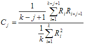
where Ri is the value of weighted residuals calculated in i-th channel; k is the number of channels where weighted residuals are calculated. The plots of autocorrelation are usually made across half of the data channels (m=k/2) were residuals are calculated. This is done in order to ensure the sufficient number of terms in the sum located in the numerator of the equation shown above thus providing the proper averaging.

In some cases the visual inspection of autocorrelation function is more sensitive test for the goodness of the fit than the plot of weighted residuals. For successful fits the residuals autocorrelation is randomly distributed around zero. Bad fits provide low frequency periodicity in an autocorrelation plot that can be detected visually.

Note: As it is follows from the equation shown above C1 = 1. This means that each Ri value is fully correlated to itself. In order to make autocorrelation plots more convenient for visual inspection in TRFA Data Processor Advanced the value C1 is replaced on the graphs by 0.

Heterosedasticity of the residuals
The graphical fit quality criterion heterosedasticity of the residuals shows the dependence of weighted residuals on the sorted ascending values of theoretical decay generated by model. For successful fits this plot should not demonstrate the broadening of one or the other side of the graph.

Normal probability density function of the residuals
This graphical fit quality criterion allows to inspect visually if weighted residuals correspond to the standard normal distribution. For this purpose the theoretical probability density function for standard normal distribution is displayed together with inspected probability density function calculated from weighted residuals. For successful fits two curves described above should be in good agreement to each other.

Analysis of single fluorescence decay

In the case if data set contains the data that correspond to separate fluorescence decay the theoretical curve is generated by the model accociated with this data set according to the equation that depends on the type of the additiobal information located in the data set.
In the case if measured data contain sample fluorescence decay and Instrumental response function all models use the following general equation:

(1)

where g(t+D) denotes the measured instrumental response function with a time shift of D relative to the sample fluorescence decay; B(t) is the measured intensity of background emission contributing with a relative weight of g; b is a level of dark noise in the instrumental response function; c is value for time-uncorrelated background photons; n is the scattered light coefficient and I(t) represents an impulse response function of the sample that is different for each individual model.

In the case if Reference compound decay has been obtained from the measurement instead of Instrumental response function all models use the following general equation:

(2)

where

denotes the measured one-exponential reference compound decay with decay time

; B(t) is the measured intensity of background emission contributing with a relative weight of g; b and c are the levels of time-uncorrelated background in reference and sample decays respectively; d(t) - Dirac delta-function.

Global analysis
The parameters of the models attached to the characteristics can be estimated by a global fitting procedure, based on the Marquardt-Levenberg non-linear method of least squares []. In the global analysis, several measured and/or simulated characteristics are combined and simultaneously fitted. Certain parameters can be linked. The values of parameters linked together are kept equal to each other.

Anisotropy analysis
The analysis of time-dependent anisotropy decays is very effective approach to study the structure of molecular systems, their behavior and processes that take place inside them. The shape of time-dependent anisotropy decays can be affected by the non-spherical form of the molecules under study, the segmental flexibility of the macromolecules, depolarization due to presence of resonance energy transfer between molecules of the same type, etc. Therefore the fit of the measured anisotropy decay to the theoretical curve generated by the model and estimation in this way the parameters that can affect the theoretical curve shape can deliver the information about the investigated molecular system.

The TRFA Data Processor Advanced software provides two approaches to perform anisotropy analysis:
1. The anisotropy analysis based on sequential fit of measured sample total fluorescence decay and measured sample parallel and perpendicular polarization components.
2. The anisotropy analysis based on direct global fit of sample parallel and perpendicular polarization components.. This approach also supports associative anisotropy analysis.

Two stage anisotropy analysis
This approach to the anisotropy analysis consists of two sequential stages and can be applied to the data sets that contain both parallel and perpendicular polarization decay components.
On the first analysis stage the measured total fluorescence decay

is calculated from parallel

and perpendicular

decay components according to the equation:

,
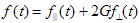(1)

where G is a G-factor that can be calculated as the ratio of emission channel sensitivity for the vertically polarized light to the emission channel sensitivity for the horizontally polarized light at the sample wavelength. Further the measured total fluorescence decay is analyzed by the model that generates theoretical curve using the general equation that depends on the type of the data located in the data set.
In the case if measured data contain sample polarization decay components and Instrumental response function polarization components

and

the theoretical curve for total fluorescence decay is calculated by the following general equation:

,
(2)

where

(3)

and I(t) represents an impulse response function of the total sample fluorescence decay that is different for each individual model;

and

are the measured parallel and perpendicular components of background emission intensity contributing with a relative weights of

and

;

and

are values for time-uncorrelated background photons in the parallel and perpendicular sample decays;

and

are the scattered light coefficients;

is the time shift in channels between

and

;

is the time shift in channels between

and

;

and

are the levels of dark noise in the parallel and perpendicular components of instrumental response function.
In the case if Reference compound decay parallel and perpendicular polarization components have been obtained from the measurement instead of

and

the theoretical curve for total fluorescence decay is calculated by the following general equation:

,
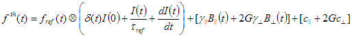(4)
where

(5)

and d(t) - Dirac delta-function;

and

denote the measured parallel and perpendicular components of one-exponential reference compound decay with decay time

. All other values in (4) and (5) are equal to corresponding values in (2) and (3).
The analysis of total fluorescence decay allows to obtain the estimations of model parameters that have an influence on the shape of the I(t).
On the second stage of anisotropy analysis parameters obtained on the previous stage can be fixed and global analysis of parallel

and perpendicular

sample decay components is performed. Since both parallel and perpendicular sample decay components are stored in one data set the theoretical curves for both of them are generated by the same model object associated with given data set. Also theoretical curves for both polarization components depend on one set of fit parameters defined by the model.
In the case if measured data contain sample polarization decay components and Instrumental response function polarization components

and

the theoretical curves for parallel and perpendicular sample decay components are calculated by the following general equations:

,
(6)
where

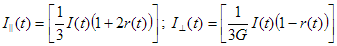
are respectively parallel and perpendicular components of impulse response function of the sample fluorescence decay and r(t) is the model-dependent function that describes the anisotropy decay.
In the case if Reference compound decay parallel and perpendicular polarization components have been obtained from the measurement instead of

and

the theoretical curves for parallel and perpendicular sample decay components are calculated by the following general equations:

.
(7)
The global analysis of parallel and perpendicular sample decay components allows to obtain the estimations of model parameters that have an influence on the shape of the

and

and thereby fit the anisotropy decay.

In order to switch between two analysis stages described above use the Experimet object property Analysis type. In the case if this property is set to Anisotropy the anisotropy decay and related dependencies can be viewed using Experiment window charts.

The models that can be used to perform the Two stage anisotropy analysis are the following:
1. Multi-exponential.

Anisotropy analysis based on the global fit
The TRFA Data Processor Advanced provides the ability to perform the anisotropy analysis as a global fit of fluorescence decays measured on the different polarization angles with respect to the exitation light.

To perform the anisotropy analysis in this way one should load the sample polarization decay components to the experiment as separate data sets. Each data set should contain the external parameter Polarization angle expressed in degrees. This external parameter is required by anisotropy model that was specially developed to perform anisotropy analysis via global fit.

The separate anisotropy model should be associated with each data set mentioned above and for all such models the parameters with the same name should be linked together. The only parameter of anisotropy model that must not be linked is the parameter A that is responsible for the fit of decay amplitude. Since the sample polarization decay components are considered as separate data sets and described with separate models the general equations that are used for generating theoretical curves by anisotropy models a the same to the equations shown in the Analysis of single fluorescence decay section. For detailed description of the equations used by anisotropy model to calculate the impulse response function of the sample I(t) please look the description of anisotropy model.

The anisotropy analysis that is performed as a global fit of fluorescence decays measured on the different polarization angles can be non-associative and associative. The required type of the anisotropy analysis can be selected with Associations property of anisotropy model.

To view the anisotropy decay and related dependencies in the case of anisotropy analysis described above the Anisotropy view window should be used.

The models that can be used to perform the Anisotropy analysis based on the global fit are the following:
1. Anisotropy.

Exhaustive search
Error estimation of the recovered parameters can be performed by the exhaustive search method (see button CI Analysis of the Configuration toolbar). In this method the examined parameter is fixed at a number of particular values in a predetermined range, while other parameters are allowed to adjust to the minimum of

. Thus, the dependence of the

values on the particular parameter is observed. Analysis stops when the calculated value of

becomes higher than the

level obtained from the statistical F-test (for that particular confidential probability and number of degrees of freedom). The value of the examined parameter obtained by the procedure described above is taken as the border of the confidential interval.
To set confidential probability use property CI Probability of the Experiment Object.

Standard errors
Error estimation of the recovered parameters can be performed by calculating asymptotic standard errors (see button CI Analysis of the Configuration toolbar).

Confidential interval for the parameter pj, j = 0, 1,… is calculated according to the following equation:

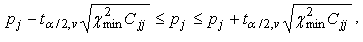
In this equation:
1. pj - the value of estimated parameter j;
2. Cjj - the jj element of the inverted Marquardt matrix obtained after the analysis;
3. a=1-b (b is confidential probability (0<b<1));
4. ta /2,v - the upper percentage point of the t - distribution (Student distribution) with v=n-p-1 degrees of freedom (n is the number of experimental points and p is the number of estimated parameters). It can be calculated from the definitions of percentage point of Student distribution and its distribution function.

5.

- the value of

obtained after the analysis.

To set confidential probability use property CI Probability of the Experiment Object.

Ratio constraint
The Ratio constraint can be added to the model in order to construct the functional relationship between model parameters that will be kept during the fit. The formula that lies in the base of Ratio constraint is the following:

where

are four sets of parameters that belong respectively to four groups (G1 - G4) shown in the formula; V is a numeric value. If no parameters have been included in one of four groups, it means that this group is absent in the formula.
Bellow several examples of possible application of Ratio constraint for multiexponential model are shown:

Functional relation between fit parameters Configuration of Ratio constraint

Sum of pre-exponential factors Group G1 contains necessary parameters. Other groups are empty. V is any number.

Difference of pre-exponential factors Groups G1 and G2 contain necessary parameters. Other groups are empty. V is any number.

Ratio of sums of pre-exponential factors Groups G1 and G3 contain necessary parameters. Other groups are empty. V is any number.

Ratio of differences of pre-exponential factors All groups contain necessary parameters. V is any number.

To configure Ratio constraint use Ratio constraint configuration dialog box that can be displayed by pressing Configure button in Add/Remove constraints dialog box.

IG type
TRFA Data Processor Advanced may use the following approaches for generating initial guesses for parameters:

IG type Description

None Generation of the initial guesses is not performed in any cases.

Empirical Generation of the initial guesses is based in the time range where measured (simulated) fluorescence decay is defined.

Phase plane method Generation of the initial guesses is performed by phase plane method [21, 22].

Default values The predefined values will be used as initial guesses. These values are specific for each type of the model and do not depend on the fluorescence decay associated with the model.

References to literature

1. J. R. Lakowicz. Principles of Fluorescence Spectroscopy. Plenum Press, New York. 1983.
2. D. V. O'Connor, D. Phillips. Time-Correlated Single Photon Counting. Academic Press, London. 1984.
3. J. N. Demas. Excited State Lifetime Measurements. Academic Press, New York. 1983.
4. G.Verbeek, A. Vaes, M. Van der Auweraer, F.C. De Schryver, C. Geelen, D. Terrell, S. De Meuter. Gaussian distributions of the decay times of the singlet excited state of aromatic amines dispersed in polymer films. Macromolecules, 26, 1993, pp. 472-478.
5. F. Imans, L. Viaene, M. Van der Auweraer, F.C. De Schryver. Local properties of adsorption sites probed by the emission of fluorophores with different size and shape. Chem. Phys. Lett., 262, 1996, pp.583-588.
6. P. P. Infelta, M. Gratzel. Dynamics of fluorescence quenching in micellar systems. J. Chem. Phys. 78, 1983, p. 5280.
7. M. Tachiya. On the kinetics of luminescence quenching in micellar systems. J. Chem. Phys, 78, 1983, p. 5282.
8. V. Van den Bergh, A. Kowalczyk, N. Boens, F.C. De Schryver. Experimental design in the Global Compartmental Analysis of Intermolecular Two-State Excited-State Processes. J. Phys. Chem., 98, 1994, pp. 9503-9508.
9. N. Boens, J. Szubiakowski, E. Novikov. Testing the identifiability of a model for reversible intermolecular two-state excited-state processes. J. Chem. Phys. 112, 2000, p. 8260.
10. A. Kowalczyk, K. Meuwis, N. Boens, F.C. De Schryver. Kinetics and Identifiability of an Intermolecular Two-State Excited-State Processes in the Presence of a Fluorescent Impurity. J. Phys. Chem., 99, 1995, pp. 17349-17353.
11. N. Boens, A. Kowalczyk. Identifiability of competitive intermolecular three-state excited-state processes. Chem. Phys. Lett., 260, 1996, pp. 326-330.
12. J. van Stam et al. Intermolecular excited-state processes of a Halato-Telechelic Polymer, Evaluated by Global Compartmental Analysis of the Fluorescence Decay Surface with the Use of Model Compounds. Macromolecules, 30, 1997, pp. 5582-5590.
13. P.R. Bevington, D.K. Robinson. Data Reduction and Error Analysis for the Physical Sciences. McGraw-Hill, New Yourk, 2003.
14. A. Grinvald, I. Z. Steinberg. On the analysis of fluorescence decay kinetics by the method of least squares. Anal. Biochem, 59, 1974, pp. 583-598.
15. Z. Bajzer, T. M. Therneau, J. C. Sharp, F. G. Prendergast. Maximum likelihood method for the analysis of time-resolved fluorescence decay curves. Eur. Biophys. J., 20, 1991, pp. 247-262.
16. D.W. Marquardt. An algorithm for least-squares estimation of non-linear parameters. J. Soc. Ind. Appl. Math., 11, 1963, pp. 431-441.
17. D.F. Eaton. Recommended methods for fluorescence decay analysis. Pure &App/Chem., Vol. 62, No. 8, 1990, pp. 1631-1648.
18. N. Boens, M. Van Den Zegel, F.C. De Schryver. Picosecond lifetime determination of the second exited singlet state of xanthione in solution. Chem. Phys. Lett., 111, 1984, pp. 340-346.
19. J. Durbin, G.C. Watson. Testing for serial correlation in least squares regression. Biometrika, 37, 1950, pp. 409-428.
20. J. R. Lakowicz. Topics in Fluorescence Spectroscopy. Vol. 2, Kluwer Academic Publishers, New York. 2002.
21. V. V. Apanasovich, E. G. Novikov. Deconvolution method for fluorescence decays. Optics communications, v. 78, 1990, pp. 279-282.
22. E. G. Novikov. Reference reconvolution analysis by phase plane method. Rev. Sci. Instr., 69, 1998, pp. 2603-2610.